MATH2331 Linear Algebra
The Class
4 quizzes (open more than 24 hours) open on Thursday
Exams are timed (65-70 minute test)
Final Exam (not cumulative) on August 19th
1.1 Introduction to Linear Systems
Background
$\mathbb{R}$ = All real numbers $(-\infty, \infty)$
$\mathbb{R}^{2}$ = xy-plane
$\mathbb{R}^{n}$ = Vector space. All $(x_1, x_2, …, x_n)$
Single variable Functions:
Linear: $f(x) = 5x,\ f(x) = ax$
Non-linear: $f(x) = x^{2} + \cos (x),\ f(x) = e^{x},\ f(x) = \tan ^{-1}(x)$
Multi-variable Functions:
Linear: $f(x,\ y) = ax + by,\ f(x,\ y,\ z) = 5x + 3y + bz$
Non-linear:
Equations:
$5 = 4x$
A linear equation in the variables $x_1,\ x_2,\ x_3,\ …,\ x_n$ is an equation of the form $a_1x_1 + a_2x_2 + x_3x_3 + … a_nx_n = b$ where $a_1,\ a_2,\ …,\ a_n$ are real numbers
A linear system (or system of linear equations) is a collection of linear equations in same variables $x_1,\ x_2,\ x_3,\ …, x_n$.
Example
$\begin{vmatrix} x & +3y & = 1 \\ x & -y & =9 \end{vmatrix} \overset{L_2 = -2 L_1 + L_2}{\implies} \begin{vmatrix} x & +3y & =1 \\ 0 & -7y & =7 \end{vmatrix} \overset{L_2 = -\frac{1}{7} L_2}{\implies} \begin{vmatrix} x & +3y & =1 \\ 0 & y & =-1 \end{vmatrix}$
$\overset{L_1 = -3 L_2 + L_1}{\implies} \begin{vmatrix} x & = 4 \\ y & = -1 \end{vmatrix}$
Example
$\begin{vmatrix} x & + 3y & =2 \\ -2x & -6y & =-4 \end{vmatrix} \overset{L_2 = 2L_1 + L_2}{\implies} \begin{vmatrix} x & +3y & = 2 \\ & 0 & = 0 \end{vmatrix}$
Solutions form the line $x+3y=2$. Infinitely many solutions.
Example
Example:
$\begin{vmatrix} x & +y & & = 0 \\ 2x & -y & + 3z & = 3 \\ x & -2y & -z & =3 \end{vmatrix} \overset{\overset{L_2 = -2L_1 + L_2}{L_3 = -L_1 + L_3}}{\implies} \begin{vmatrix} x & +y & &=0 \\ & -3y & +3z & = 3 \\ & -3y & -z & =3 \end{vmatrix}$
$\overset{L_2 = L_2 -\frac{1}{3}}{\implies} \begin{vmatrix} x & +y & & = 0 \\ & y & -z & =-1 \\ & & z & =0 \end{vmatrix} \overset{L_3 = 3L_2 + L_3}{\implies} \begin{vmatrix} x & +y & & =0 \\ & y & -z & -1 \\ & & -4z & = 0 \end{vmatrix}$
$\overset{L_3 = -\frac{1}{4} L_3}{\implies} \begin{vmatrix} x & +y & =0 \\ & y & -z & = -1 \\ & & z & =0 \end{vmatrix} \overset{L_2 = L_3 + L_2}{\implies} \begin{vmatrix} x & + y & & =0 \\ & y & & =-1 \\ & & z & =0 \end{vmatrix}$
$\overset{L_1 = L_1 - L_2}{\implies} \begin{vmatrix} x & =1 \\ y & =-1 \\ z &=0 \end{vmatrix}$
Solution $(x,\ y,\ z) = (1,\ -1,\ 0)$
Example
$\begin{vmatrix} x & + y & + z & =2 \\ & y & +z & =1 \\ x & +2y & 2z & =3 \end{vmatrix} \overset{L_3 = -L_1 + L_3}{\implies} \begin{vmatrix} x & +y & +z & = 2 \\ & y & + z & =1 \\ & y & +z & =1 \end{vmatrix}$
$\overset{L_3 = -L_2 + l_3}{\implies} \begin{vmatrix} x & +y & +z & =2 \\ & y & +z & =1 \\ & & 0 & =0 \end{vmatrix} \overset{L_1 = -L_2 + L_1}{\implies} \begin{vmatrix} x & & & =1\\ & y & +z & =1\\ & & 0 & =0 \end{vmatrix}$
This example has a free variable. Let $z=t$.
Solution: $(x,\ y,\ z) = (1,\ 1-t,\ t)$. Has infinitely many solutions.
$y + z = 1 \implies y = 1 -t$
Example
$\begin{vmatrix} x & + y & + z & =2 \\ & y & + z & =1 \\ & 2y & + 2z & =0 \end{vmatrix} \overset{L_3 = -2L_2 + L_3}{\implies} \begin{vmatrix} x & +y & +z & =2 \\ & y & + z & =1 \\ & & 0 & =-2 \end{vmatrix}$
No solutions.
How many solutions are possible to a system of linear equations?
Answer:
- 0 Solutions
- 1 Solution
- Infinitely many solutions
(This is because planes cannot curve)
Geometric Interpretation
A linear equation $ax + by = c$ defined a line in $\mathbb{R}^{2}$
Solutions to a linear system are intersections of lines in $\mathbb{R}^{2}$.
- 0 Points (Solutions)
- 1 Point (Solution)
- $\infty$ many points (Solutions) if they are the same line
A linear equation $ax + by + cz = d$ defined a plane in $\mathbb{R}^{3}$.
Solutions to a linear system are intersections of (hyper) planes in $\mathbb{R}^{3}$.
- 0 Points (Solutions)
- 1 Point (Solution)
- $\infty$ many points (Solutions): All the planes contain a line. Also if all planes could be the same plane.
Example
Find all polynomials $f(t)$ of degree $\le 2$.
- Whose graph run through (1, 3) and (2, 6) and
- Such that $f^{\prime}(1) = 1$
- Use $f(t) = a + bt + ct^{2}$
We know
- $f(1) = 3 \implies a + b + c = 3$
- $f(2) = 6 \implies a + 2b + 4c = 6$
- $f’(t) = b + 2ct$
- $f’(1) = 1 \implies b + 2c = 1$
$\begin{vmatrix} a & +b & + c & =3 \\ a & +2b & +4c & =6 \\ & b & +2c & =1 \end{vmatrix} \overset{L_2 = -L_1 + L_2}{\implies} \begin{vmatrix} a & +b & +c & =3\\ & b & +3c & =3 \\ & b & +2c & =1 \end{vmatrix}$
$\overset{L_3 = -L_2 + L_3}{\implies} \begin{vmatrix} a & +b & +c & =3 \\ & b& +3c & =3 \\ & & c & =2 \end{vmatrix} \overset{\overset{L_2 = -3L_3 + L_2}{L_1 = -L_3 + L_1}}{\implies} \begin{vmatrix} a & +b & =1\\ & b & -3\\ & c & =2 \end{vmatrix}$
$\overset{L_1 = L_1 - L_2}{\implies} \begin{vmatrix} a & =4 \\ b & =-3 \\ c & =2 \end{vmatrix}$
$f(t) = 4 - 3t + 2t^{2}$
1.2 Matrices, Vectors, and Gauss-Jordan Elimination
$\begin{vmatrix} x & +2y & +3z & =1 \\ 2x & +4y & +7z & =2 \\ 3x & +7y & +4z & =8 \end{vmatrix}$
We can store all information in this linear system in a matrix which is a rectangular array of numbers.
Augmented Matrix:
$\begin{bmatrix} 1 & 2 & 3 & \bigm| & 1 \\ 2 & 4 & 7 & \bigm| & 2 \\ 3 & 7 & 11 & \bigm| & 8 \end{bmatrix} $
3 row and 4 column = 2x4 matrix
Coefficient Matrix:
$\begin{bmatrix} 1 & 2 & 3 \\ 2 & 4 & 7 \\ 3 & 7 & 1 \end{bmatrix}$
3 x 3 matrix
Generally, we have
$A = [a_{ij}] = \begin{bmatrix} a_{11} & a_{12} & a_{13} & \cdots & a_{1m} \\ a_{21} & a_{22} & a_{23} & \cdots & a_{2m} \\ \vdots & \vdots & \vdots & \ddots & \vdots \\ a_{n_1} & a_{n2} & a_{n3} & \cdots & a_{nm} \end{bmatrix} $
Here, $A$ is $n\times m$ (n rows and m columns).
For square $n \times n$ matrices:
Diagonal: $a_{ij}$ for $i \neq j$
Lower triangular: $a_{ij} = 0$ for $i < j$
Upper triangular: $a_{ij} = 0$ for $i > j$
Identity matrix $I_n$: square $n\times n$ diagonal ($a_{ij} = 0$ for $i \neq j$ ) and $a_{ii} = 1$ for $1 \le i = n$
$I_3 = \begin{bmatrix} 1 & 0 & 0 \\ 0 & 1 & 0 \\ 0 & 0 & 1 \end{bmatrix} $
0 Matrix: Any size; all entries are 0
$\begin{bmatrix} 0 & 0 & 0 & 0 & 0 \\0 & 0 & 0 & 0 & 0 \end{bmatrix}$
Above is a $2\times 5$ 0-Matrix
Columns of an $n \times m$ matrix form vectors in $\mathbb{R}^{n}$. Example:
\[\begin{bmatrix} 1 & 2 & 3 & \Bigm| & 1 \\ 2 & 4 & 7 & \Bigm| & 2 \\ 3 & 7 & 11 & \Bigm| & 8 \end{bmatrix}\]We can represent vectors as the columns:
\[\begin{bmatrix} 1 \\ 2 \end{bmatrix} , \begin{bmatrix} 3 \\ 1 \end{bmatrix} , \begin{bmatrix} 1 \\ 9 \end{bmatrix} , \text{ in } \mathbb{R}^2\]This is the standard representation for a vector in $\mathbb{R}^{n}$. A vector as an arrow starting at origin and ending at corresponding point.
Consider the two vectors:
\[\vec{v} = \begin{bmatrix} 1 \\ 2 \end{bmatrix} , \vec{w} = \begin{bmatrix} 3 \\ 1 \end{bmatrix} \text{ in } \mathbb{R}^2\]
We may use 3 elementary row operations
- Multiply/divide a row by a nonzero constant
- Add/subtract a multiple of one row to another
- Interchange two rows
Solving the system of linear equations:
Example
\[\begin{bmatrix}
1 & 2 & 3 & \Bigm| & 1 \\
2 & 4 & 7 & \Bigm| & 2 \\
3 & 7 & 11 & \Bigm| & 8
\end{bmatrix}
\overset{\overset{-2R_1 + R2}{-3R_1 + R_3}}{\implies}
\begin{bmatrix}
1 & 2 & 3 & \Bigm| & 1 \\
0 & 0 & 1 & \Bigm| & 0 \\
0 & 1 & 2 & \Bigm| & 5 \\
\end{bmatrix}
\overset{R_2 \leftrightarrow R_3}{\implies}
\begin{bmatrix}
1 & 2 & 3 & \bigm| & 1 \\
0 & 1 & 2 & \bigm| & 5 \\
0 & 0 & 1 & \bigm| & 0
\end{bmatrix}\]
\[\overset{\overset{-3R_3 + R_1}{-2R_3 + R_2}}{\implies}
\begin{bmatrix}
1 & 2 & 0 & \bigm| & 1 \\
0 & 1 & 0 & \bigm| & 5 \\
0 & 0 & 1 & \bigm| & 0
\end{bmatrix}
\overset{-2R_2 + R_1}{\implies}
\begin{bmatrix}
1 & 0 & 0 & \bigm| & -9 \\
0 & 1 & 0 & \bigm| & 5 \\
0 & 0 & 1 & \bigm| & 0
\end{bmatrix}
\text{ identity matrix}\]
\[\therefore
\begin{bmatrix}
x \\
y \\
z
\end{bmatrix}
=
\begin{bmatrix}
-9 \\
5 \\
0
\end{bmatrix}\]
Example
\[\begin{bmatrix}
1 & -1 & 1 & \bigm| & 0 \\
1 & 0 & -2 & \bigm| & 2 \\
2 & -1 & 1 & \bigm| & 4 \\
0 & 2 & -5 & \bigm| & 4
\end{bmatrix}
\overset{\overset{-R_1 + R_2}{-2R_1 + R_3}}{\implies}
\begin{bmatrix}
1 & -1 & 1 & \bigm| & 0 \\
0 & 1 & -3 & \bigm| & 2 \\
0 & 1 & -1 & \bigm| & 4 \\
0 & 2 & -5 & \bigm| & 4
\end{bmatrix}\]
\[\overset{\overset{-R_2 + R_3}{-2R_2 + R_4}}{\implies}
\begin{bmatrix}
1 & -1 & 1 & \bigm| & 0 \\
0 & 1 & -3 & \bigm| & 2 \\
0 & 0 & 2 & \bigm| & 2 \\
0 & 0 & 1 & \bigm| & 0 \\
\end{bmatrix}
\overset{R_3 \leftrightarrow R_4}{\implies}
\begin{bmatrix}
1 & -1 & 1 & \bigm| & 0 \\
0 & 1 & -3 & \bigm| & 2 \\
0 & 0 & 1 & \bigm| & 0 \\
0 & 0 & 2 & \bigm| & 2 \\
\end{bmatrix}\]
\[\overset{-2R_3 + R_4}{\implies}
\begin{bmatrix}
1 & -1 & 1 & \bigm| & 0 \\
0 & 1 & -3 & \bigm| & 2 \\
0 & 0 & 1 & \bigm| & 0 \\
0 & 0 & 0 & \bigm| & 2 \\
\end{bmatrix}\]
No solutions
Example
\[\begin{bmatrix}
x_1 & x_2 & x_3 & x_4 & x_5 \cdots \\
\vdots & \vdots & \vdots & \vdots & \ddots
\end{bmatrix}
=
\begin{bmatrix}
1 & -7 & 0 & 0 & 1 & \bigm| & 3 \\
0 & 0 & 1 & 0 & -2 & \bigm| & 2 \\
0 & 0 & 0 & 1 & 1 & \bigm| & 1
\end{bmatrix}\]
This is already as far as we can go with row operations, but we have two free variables. They are $x_2$ and $x_5$.
We can say that
$x_2 = t$
$x_5 = s$
$x_1 = 3 + 7t - s$
$x_3 = 2 + 2s$
$x_4 = 1 - s$
\[\begin{bmatrix} x_1 \\ x_2 \\ x_3 \\ x_4 \\ x_5 \end{bmatrix} = \begin{bmatrix} 3 + 7t - 5 \\ t \\ 2 + 2s \\ 1 - s \\ s \end{bmatrix}\]
Example
\[\begin{bmatrix}
1 & 1 & 2 & \bigm| 0 \\
2 & -1 & 1 & \bigm| 6 \\
4 & 1 & 5 & \bigm| 6 \\
\end{bmatrix}
\overset{\overset{-R_1 + R_2}{-4R_1 + R_3}}{\implies}
\begin{bmatrix}
1 & 1 & 2 & \bigm| & 0 \\
0 & -3 & -3 & \bigm| & 6 \\
0 & -3 & -3 & \bigm| & 6
\end{bmatrix}\]
\[\overset{\left( -\frac{1}{3} \right) R_2}{\implies}
\begin{bmatrix}
1 & 1 & 2 & \bigm| & 0 \\
0 & 1 & 1 & \bigm| & -2 \\
0 & -3 & -3 & \bigm| & 6
\end{bmatrix}
\overset{3R_2 + R_3}{\implies}
\begin{bmatrix}
1 & 1 & 2 & \bigm| & 0 \\
0 & 1 & 1 & \bigm| & -2 \\
0 & 0 & 0 & \bigm| & 0
\end{bmatrix}\]
\[\overset{-R_2 + R_1}{\implies}
\begin{bmatrix}
1 & 0 & 1 & \bigm| & 2 \\
0 & 1 & 1 & \bigm| & -2 \\
0 & 0 & 0 & \bigm| & 0
\end{bmatrix}\]
$z=t$ (free variable)
$x = 2-t$
$y= -3 - t$
\[\begin{bmatrix} x \\ y \\ z \end{bmatrix} = \begin{bmatrix} 2 -t\\ -2-t\\ t \end{bmatrix}\]Reduced Row Echelon Form (rref)
Defintion: An $n\times m$ matrix is in reduced row echelon form (rref) provided:
- If a row has nonzero entries, the first nonzero entry is a 1, called leading 1 or pivot.
- If a column contains a leading 1, then all other entries in column are zero.
- If a row contains a leading 1,then each row above has a leading 1 and to the left.
Examples of matrices in reduced row echelon form:
\[\begin{bmatrix} 1 & -7 & 0 & 0\\ 0 & 0 & 1 & 0 \\ 0 & 0 & 0 & 1 \\ 0 & 0 & 0 & 0 \end{bmatrix} , \begin{bmatrix} 1 & 0 & 5 & 2\\ 0 & 1 & 2 & 7 \\ 0 & 0 & 0 & 0 \\ \end{bmatrix} , \begin{bmatrix} 1 & 2 & 5 \\ 0 & 0 & 0 \\ 0 & 0 & 0 \\ 0 & 0 & 0 \\ 0 & 0 & 0 \end{bmatrix} , \begin{bmatrix} 0 & 0 & 1 & 0 \\ 0 & 0 & 0 & 1 \\ 0 & 0 & 0 & 0 \\ 0 & 0 & 0 & 0 \\ \end{bmatrix}\]Row echelon form (ref)
Differences:
- Leading entry (pivot position) in a row can be anything
- No restriction on entries above a leading entry in a column
Using the 3 elementary row operations, we may transform any matrix to one in rref (also ref). This method of solving a linear system is called Guass-Jordan Elimination.
1.3 On the Solutions of Linear Systems: Matrix Algebra
Consider the augmented matrices:
ref with 1 unique solution: $\begin{bmatrix} 2 & 0 & 0 & \bigm| & -3 \\ 0 & 3 & 0 & \bigm| & 3 \\ 0 & 0 & 1 & \bigm| & 14\end{bmatrix} $
rref with infinitely many solutions: $\begin{bmatrix} 1 & 0 & 0 & 0 & 1 & \bigm| & -1 \\ 0 & 1 & 0 & 0 & 1 & \bigm| & 0 \\ 0 & 0 & 1 & 1 & 0 & \bigm| & 2\end{bmatrix} $
ref with 1 unique solution: $\begin{bmatrix} 0 & 0 & 0 & \bigm| & 4 \\ 0 & 1 & 2 & \bigm| & 4 \\ 0 & 0 & 3 & \bigm| & 6 \\ 0 & 0 & 0 & \bigm| & 0 \\ 0 & 0 & 0 & \bigm| & 0 \\ \end{bmatrix}$
ref with no solutions: $\begin{bmatrix} 1 & 0 & 0 & \bigm| & 3 \\ 0 & 1 & 0 & \bigm| & -1 \\ 0 & 0 & 2 & \bigm| & 4 \\ 0 & 0 & 0 & \bigm| & 10 \\ \end{bmatrix}$
A linear system is
- consistent provided it has at least one solution
- inconsistent provided it has no solutions
Theorem:
- A linear system is inconsistent if and only if a row echelon form (ref) of its augmented matrix has a row $\begin{bmatrix} 0 & 0 & 0 & \cdots & 0 & \bigm| & c \end{bmatrix}$ where $c\neq 0$.
- A linear system is consistent then we have either:
- A unique solution or
- Infinitely many solutions (at least one free variable)
Rank
The rank of a matrix $A$, denoted rank(A) is the number of leading 1’s in rref(A) (the reduced row echelon form of $A$).
Example
ref
\[\begin{bmatrix} 2 & 0 & 0\\ 0 & 3 & 0 \\ 0 & 0 & 1 \end{bmatrix}\]Has a rank of 3 (3x3)
Example
rref:
\[\begin{bmatrix} 1 & 0 & 0 & 0 & 1 \\ 0 & 1 & 0 & 0 & 1 \\ 1 & 0 & 1 & 1 & 0 \\ \end{bmatrix}\]Has a rank of 3 (3x5)
Example
ref: \(\begin{bmatrix} 1 & 0 & 0 \\ 0 & 1 & 2 \\ 0 & 0 & 3 \\ 0 & 0 & 0 \\ 0 & 0 & 0 \\ \end{bmatrix}\)
Rank of 3 (5x3)
Example
rref: \(\begin{bmatrix} 1 & 0 & 0 \\ 0 & 0 & 0 \\ 0 & 0 & 0 \\ \end{bmatrix}\)
Rank of 1 (3x3)
Example
rref: \(\begin{bmatrix} 0 & 0 & 1 & 0 & 1 & 0 \\ 0 & 0 & 0 & 1 & 4 & 0 \\ 0 & 0 & 0 & 0 & 0 & 1 \\ 0 & 0 & 0 & 0 & 0 & 0 \\ \end{bmatrix}\)
rank of 3 (4x6 matrix)
Example
\[\begin{bmatrix}
3 & 3 & 3 \\
3 & 3 & 3
\end{bmatrix}
\overset{\frac{1}{3} R_1}{\implies}
\begin{bmatrix}
1 & 1 & 1 \\
3 & 3 & 3
\end{bmatrix}
\overset{-3R_1 + R_2}{\implies} \text{rref}:
\begin{bmatrix}
1 & 1 & 1 \\
0 & 0 & 0
\end{bmatrix}\]
This matrix has a rank of 1.
Example
\[\begin{bmatrix}
1 & 1 & 1 \\
1 & 2 & 3 \\
1 & 3 & 6 \\
0 & 0 & 0
\end{bmatrix}
\overset{\overset{R_2 - R_1}{-R_1 + R_3}}{\implies}
\begin{bmatrix}
1 & 1 & 1 \\
0 & 1 & 2 \\
0 & 2 & 5 \\
0 & 0 & 0
\end{bmatrix}
\overset{R_3 - 2R_2}{\implies}
\begin{bmatrix}
1 & 1 & 1 \\
0 & 1 & 2 \\
0 & 0 & 1 \\
0 & 0 & 0
\end{bmatrix}\]
The rank of this matrix is 3.
Example
\[C =
\begin{bmatrix}
0 & 1 & a \\
-1 & 0 & b \\
-a & -b & 0
\end{bmatrix}
\overset{R_1 \leftrightarrow R_2}{\implies}
\begin{bmatrix}
-1 & 0 & b \\
0 & 1 & a \\
-a & -b & 0
\end{bmatrix}
\overset{-1 \times R_1}{\implies}
\begin{bmatrix}
1 & 0 & -b \\
0 & 1 & a \\
-a & -b & 0
\end{bmatrix}\]
\[\overset{aR_1 + R_3}{\implies}
\begin{bmatrix}
1 & 0 & -b \\
0 & 1 & a \\
0 & -b & -ab
\end{bmatrix}
\overset{bR_2 + R_3}{\implies}
\begin{bmatrix}
1 & 0 & -b \\
0 & 1 & a \\
0 & 0 & 0
\end{bmatrix}\]
Rank is 2.
Suppose we have an $n \times m$ coefficeint matrix
\[A = \begin{bmatrix} a_{11} & a_{12} & \cdots & a_{1m} \\ a_{21} & a_{22} & \cdots & a_{2m} \\ \vdots & \vdots & \ddots & \vdots \\ a_{n1} & a_{n2} & \cdots & a_{nm} \end{bmatrix}\]$\text{rank}(A) \le n$
$\text{rank}(A) \le m$
Number of free variables = $m - \text{rank}(A)$
If a linear system with coefficient matrix $A$ has:
- exactly one solution, then we have no free variables. Therefore the $\text{rank}(A) = m$.
- no solutions, then ret augmented matrix $\begin{bmatrix} 0 & 0 & 0 & \big| & b \end{bmatrix} $ where $b\neq 0$. Therefore $\text{rank(A)} < n$.
- infinitely many solutions, then at least one free variable $\text{rank(A)} < m$.
Square Matricies: When a linear system has an $n \times n$ coefficient matrix $A$, there is exactly one soltuion…
if and only if $\text{rank}(A) = n$
if and only if $\text{rref}(A) = I_n$ (the $n \times n$ identity)
Matrix Algebra
Suppose $A = [a_{ij}]$ and $B = [b_{ij}]$ are both $n \times m$ and $c$ is in $\mathbb{R}$.
Matrix Sum: $A+B = [a_{ij} + b_{ij}]$ (add/scalar multiply entry by entry)
Scaler Multiplication: $cA = [ca_{ij}]$
Example
\[\begin{bmatrix}
2 & 3 \\
5 & -2 \\
-1 & 0
\end{bmatrix}
+
\begin{bmatrix}
-1 & 6 \\
3 & 0 \\
0 & 2
\end{bmatrix}
=
\begin{bmatrix}
1 & 9 \\
8 & -2 \\
-1 & 2
\end{bmatrix}\]
Example
\[5
\begin{bmatrix}
2 & 3 & -1 \\
1 & 3 & -3
\end{bmatrix}
=
\begin{bmatrix}
10 & 15 & -5 \\
5 & 15 & -15
\end{bmatrix}\]
Example
Vector Sum and Scaler multiplication
\[\vec{v} = \begin{bmatrix} 4\\ 3 \\ 1 \end{bmatrix}\] \[\vec{w} = \begin{bmatrix} 0 \\ 1 \\ -1 \end{bmatrix}\] \[\vec{v} + \vec{w} = \begin{bmatrix} 4 \\ 4 \\ 0 \end{bmatrix}\]What about matrix/vector products?
- Dot product for 2 vectors in $\mathbb{R}^n$
- $A \vec{x}$ matrix times vector
Definition:
For vectors $\vec{v} = \begin{bmatrix} v_1 \\ v_2 \\ \vdots \\ v_n \end{bmatrix} $ and $\vec{w} = \begin{bmatrix} w_1 \\ w_2 \\ \vdots \\ w_n \end{bmatrix} $ in $\mathbb{R}^n$, the dot product $\vec{v} * \vec{w}$ is scaler:
$\vec{v} * \vec{w} = v_1 w_1 + v_2 w_2 + v_3 w_3 … = \sum_{k=1}^{n} v_k w_k$
Note: dot product does not distinguish between row vectors and column vectors.
Example
\[\begin{bmatrix}
5 \\
2 \\
-3
\end{bmatrix}
*
\begin{bmatrix}
1 \\
-1 \\
-1
\end{bmatrix}
= 5 * 1 + 2(-1) + (-3)(-1) = 5 +2 + 3 = 6\]
An important way to think about dot product:
\[\begin{bmatrix} 5 & 2 & -3 \end{bmatrix} \begin{bmatrix} 1 \\ -1 \\ -1 \end{bmatrix}\]The product $A\vec{x}$ : Suppose $A$ is $n\times m$ and $\vec{x} = \begin{bmatrix} x_1 \\ x_2 \\ \vdots \\ x_m \end{bmatrix} $
Size: $\left( n\times m \right) \left( m \times 1\right) \to n \times 1$
Way 1: Row Viewport
\[A = \begin{bmatrix} -- \vec{w_1} -- \\ -- \vec{w_2} -- \\ \vdots \\ -- \vec{w_n} -- \\ \end{bmatrix}\]Note: $\vec{w}_i \in \mathbb{R}^m$
\[A\vec{x} = \begin{bmatrix} \vec{w_1} * \vec{x} \\ \vec{w_2} * \vec{x} \\ \vdots \\ \vec{w_n} * \vec{x} \end{bmatrix}\](Size $n \times 1$)
Way 2: Column Viewport
\[A = \begin{bmatrix} | & | & & | \\ \vec{v_1} & \vec{v_2} & \cdots & \vec{v_m} \\ | & | & & | \\ \end{bmatrix}\]$\vec{v_j} \in \mathbb{R}^n$
$A \vec{x} = x_1 \vec{v_1} + x_2 \vec{v_2} + \cdots + x_m \vec{v_m}$
(Size $n \times 1$)
Example
\[\begin{bmatrix}
5 & -1 & 2 & 6 \\
4 & 3 & 0 & 1 \\
-1 & 0 & 2 & -1
\end{bmatrix}
\begin{bmatrix}
0 \\
2 \\
-1 \\
3
\end{bmatrix}
=\]
\[0
\begin{bmatrix}
5 \\
4 \\
-1
\end{bmatrix}
+
2 \begin{bmatrix}
-1 \\
3 \\
0
\end{bmatrix}
- 1
\begin{bmatrix}
2 \\
0 \\
2
\end{bmatrix}
+ 3
\begin{bmatrix}
6 \\
1 \\
-1
\end{bmatrix}
=
\begin{bmatrix}
14 \\
9 \\
-5
\end{bmatrix}\]
Example
\[\begin{bmatrix}
5 & -1 & 2 & 6 \\
4 & 3 & 0 & 1 \\
-1 & 0 & 2 & -1
\end{bmatrix}
\begin{bmatrix}
2 \\
3 \\
2
\end{bmatrix}\]
Product is not defined
Example
\[\begin{bmatrix}
5 & -2 \\
3 & 1 \\
1 & 4 \\
-1 & 0 \\
0 & 6
\end{bmatrix}
\begin{bmatrix}
2 \\
-1
\end{bmatrix}
=
\begin{bmatrix}
10 + 2 \\
6 - 1 \\
2 - 4 \\
-2 + 0 \\
0 - 6
\end{bmatrix}
=
\begin{bmatrix}
12 \\
5 \\
-2 \\
-2 \\
-6
\end{bmatrix}\]
Definition:
A vector $\vec{b}$ in $\mathbb{R}^n$ is a linear combination of $\vec{v_1},\ \vec{v_2},\ \cdots,\ \vec{v_m}$ in $\mathbb{R}^n$ provided there exists scalars $x_1,\ x_2,\ x_3,\ \cdots ,\ x_m$ with $\vec{b} = x_1 \vec{v_1} + x_2 \vec{v_2} + x_3 \vec{v_3} + \cdots + x_m \vec{v_m}$.
Example
$\begin{bmatrix} 4 \\ 10 \\ 2 \\ -3 \end{bmatrix} $ is a linear combination of $\begin{bmatrix} 0 \\ 2 \\ 0 \\ -1 \end{bmatrix}$ and $\begin{bmatrix} 2 \\ 0 \\ 1 \\ 1 \end{bmatrix}$
\[\begin{bmatrix} 4 \\ 10 \\ 2 \\ -3 \end{bmatrix} = 5 \begin{bmatrix} 0 \\ 2 \\ 0 \\ -1 \end{bmatrix} + 2 \begin{bmatrix} 2 \\ 0 \\ 1 \\ 1 \end{bmatrix}\]
Example
$\begin{bmatrix} 4 \\ 10 \\ 2 \\ -3 \end{bmatrix} $ is a linear combination of $\vec{e_1} = \begin{bmatrix} 1 \\ 0 \\ 0 \\ 0 \end{bmatrix} $, $\vec{e_2} = \begin{bmatrix} 0 \\ 1 \\ 0 \\ 0 \end{bmatrix} $, $\vec{e_3} = \begin{bmatrix} 0 \\ 0 \\ 1 \\ 0 \end{bmatrix}$, and $\vec{e_4} = \begin{bmatrix} 0 \\ 0 \\ 0 \\ 1 \end{bmatrix}$.
In $\mathbb{R}^n$ vector, for $1 \le i \le n$ : $\vec{e_i}$ has 1 in $i$th spot and 0 elsewhere.
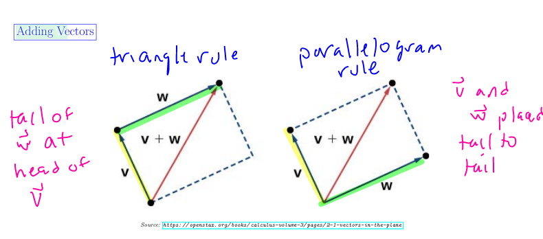
\[\begin{bmatrix} 4 \\ 10 \\ 2 \\ -3 \end{bmatrix} = 4 \vec{e_1} + 10 \vec{e_2} + 2 \vec{e_3} - 3 \vec{e_4}\]Adding vectors with parallelogram rule

Example
$\begin{bmatrix} 0 \\ 0 \\ 1 \end{bmatrix}$ in $\mathbb{R}^3$ is not linear combination of $\vec{e_1}$ and $\vec{e_2}$. Linear combinations of $\vec{e_1}$ and $\vec{e_2}$ just fill out the xy-plane. It cannot traverse the z-axis.
Example
Let $\vec{b} = \begin{bmatrix} 4 \\ 10 \\ 2 \\ -3 \end{bmatrix}$. Is $\vec{b}$ a linear combination of $\vec{v} = \begin{bmatrix} 4 \\ 2 \\ 1 \\ -1 \end{bmatrix}$ and $\vec{w} = \begin{bmatrix} 2 \\ -1 \\ 1 \\ 1 \end{bmatrix}$
What we want: scalars $x_1$, $x_2$ with:
\[x_1 \begin{bmatrix} 4 \\ 2 \\ 1 \\ -1 \end{bmatrix} + x_2 \begin{bmatrix} 2 \\ -1 \\ 1 \\ 1 \end{bmatrix} = \begin{bmatrix} 4 \\ 10 \\ 2 \\ -3 \end{bmatrix}\](We will finish this next lecture)
Quiz 1 Preparation
Example
Solve the linear system by elementary row operations.
\[\begin{bmatrix} 1 & 6 & 2 & -5 & \big| & 3 \\ 0 & 0 & 2 & -8 & \big| & 2 \\ 1 & 6 & 1 & -1 & \big| & 2 \end{bmatrix} \overset{-R_1 + R_2}{\implies} \begin{bmatrix} 1 & 6 & 2 & -5 & \big| & 3 \\ 0 & 0 & 2 & -8 & \big| & 2 \\ 0 & 0 & -1 & -4 & \big| & 2 \end{bmatrix}\] \[\overset{\frac{1}{2} R_2}{\implies} \begin{bmatrix} 1 & 6 & 2 & -5 & \big| & 3 \\ 0 & 0 & 1 & -4 & \big| & 1 \\ 0 & 0 & -1 & -4 & \big| & 2 \end{bmatrix} \overset{R_2 + R_3}{\implies} \begin{bmatrix} 1 & 6 & 2 & -5 & \big| & 3 \\ 0 & 0 & 1 & -4 & \big| & 1 \\ 0 & 0 & 0& 0 & \big| & 2 \end{bmatrix}\] \[\overset{-R_1 + R_1}{\implies} \begin{bmatrix} 1 & 6 & 0 & 3 & \big| & 1 \\ 0 & 0 & 1 & -4 & \big| & 1 \\ 0 & 0 & 0& 0 & \big| & 2 \end{bmatrix}\]$x_2 = 5$
$x_4 = 5$
$x_1 = 1 - 6s - 3t$
$x_3 = 1 + 4t$
\[\begin{bmatrix} x_1 \\ x_2 \\ x_3 \\ x_4 \end{bmatrix} = \begin{bmatrix} 1-6s-3t \\ s \\ 1+4t \\ t \end{bmatrix}\]
Example
Find all polynomails of the form $f(t) = a + bt + ct^2$ with the point (1, 6) on the graph of $f$ such that $f’(2) = 9$ and $f’‘(8) = 4$.
$f’(t) = b + 2ct$
$f’‘(t) = 2c$
$f(1) = 6 \to a + b + c = 6$
$f’(2) = 9 \to b + 4c = 9$
$f’‘(8) = 4 \to 2c = 4$
$c = 2$
$b + 2 = 9 \implies b = 1$
$a + 1 + 2 = 6 \implies a=3$
$f(t) = 3 + t + 2t^2$
Example
Find one value $c$ so that the agumented matrix below corresponds to an inconsistent linear system.
\[\begin{bmatrix} 1 & 2 & -1 & \big| & 3 \\ 2 & 4 & -2 & \big| & c \end{bmatrix}\]Note that in order for an inconsistent linear system, you need the form: $\begin{bmatrix} 0 & 0 & 0 & \big| & b \end{bmatrix} $
\[\begin{bmatrix} 1 & 2 & -1 & \big| & 3 \\ 2 & 4 & -2 & \big| & c \end{bmatrix} \overset{2R_1 - R_2}{\implies} \begin{bmatrix} 1 & 2 & -1 & \big| & 3 \\ 0 & 0 & 0 & \big| & 6 - c \end{bmatrix}\]So when $c \neq 6$.
Example
Consider the matriceis $A$, $B$, $C$, $D$ below.
\[A = \begin{bmatrix} 1 & 3 & 0 & -1 & 5 \\ 0 & 1 & 0 & 9 & 0 \\ 0 & 0 & 0 & 0 & 0 \\ 0 & 0 & 1 & 1 & 4 \\ \end{bmatrix}\] \[B = \begin{bmatrix} 0 & 1 & 6 & 0 & 3 & -1 \\ 0 & 0 & 0 & 1 & 2 & 2 \\ 0 & 0 & 0 & 0 & 0 & 0 \end{bmatrix}\] \[C = \begin{bmatrix} 0 & 1 & 0 & 2 & 4 \end{bmatrix}\] \[D = \begin{bmatrix} 0 \\ 1 \\ 0 \\ 2 \\ 4 \end{bmatrix}\]a) Which of the matrices are in reduced row-echelon form (rref)?
Solution
B, C
b) List the rank of each matrix
Solution
rank($A$) = 3
rank($B$) = 2
rank($C$) = rank($D$) = 1
A linear system is consistent if and only if rank of coefficient matrix equals tank of augmented matrix. For example, this would change the rank:
\[\begin{bmatrix} \vdots & \big\| & \vdots \\ 0 & \big\| & 1 \end{bmatrix}\]Recall
$A \vec{x}$ for $A$ an $n \times m$ matrix and $\vec{x} = \begin{bmatrix} x_1 \\ \vdots \\ x_m \end{bmatrix} $
Row Viewport:
Suppose $\vec{w_1}, \vec{w_2}, \cdots, \vec{w_n}$ in $\mathbb{R}^m$ are the rows of $A$, then:
\[A\vec{x} = \begin{bmatrix} - & \vec{w_1} * \vec{x} & - \\ - & \vec{w_2} * \vec{x} & - \\ & \vdots & \\ - & \vec{w_m} * \vec{x} & - \\ \end{bmatrix}\]ith entry of $A \vec{x}$ is [Row i of $A$] $\cdot \vec{x}$
Column Viewport:
Suppose $\vec{v_1},\ \vec{v_2},\ \cdots ,\ \vec{v_m}$ in $\mathbb{R}^n$ are ithe columns of $A$, i.e. $A = \begin{bmatrix} | & | && | \\ \vec{v_1} & \vec{v_2} & \cdots & \vec{v_m} \\ | & | && | \end{bmatrix} $
Then, $A \vec{x} = x_1 \vec{v_1} + x_2 \vec{v_2} + \cdots + x_m \vec{v_m}$
Properties of the product $A\vec{x}$: Suppose $A$ is $n\times m$, $\vec{x}$, $\vec{y}$ are in $\mathbb{R}^m$ and $k$ is a scalar
- $A(\vec{x} + \vec{y}) = A\vec{x} + A\vec{y}$
- $A(k\vec{x}) = kA\vec{x}$
Justification of 2:
$k\vec{x} = \begin{bmatrix} kx_1 \\ kx_2 \\ \vdots \\ kx_m \end{bmatrix}$
$A(k\vec{x}) = (kx_1) \vec{v_1} + (kx_2)\vec{v_2} + \cdots + (kx_m) \vec{v_m}$
$= k(x_1 \vec{v_1} + x_2 \vec{v_2} + \cdots + x_m \vec{v_m})$
$= kA\vec{x}$
We continue with this question: is $\begin{bmatrix} 4 \\ 10 \\ 2 \\ -3 \end{bmatrix}$ a linear combination of $\begin{bmatrix} 4 \\ 2 \\ 1 \\ -1 \end{bmatrix}$ and $\begin{bmatrix} 2 \\ -1 \\ 1 \\ 1 \end{bmatrix}$?
Can we find $x_1$, $x_2$ scalars such that $x_1 \begin{bmatrix} 4 \\ 2 \\ 1 \\ -1 \end{bmatrix} + x_2 \begin{bmatrix} 2 \\ -1 \\ 1 \\ 1 \end{bmatrix} = \begin{bmatrix} 4 \\ 10 \\ 2 \\ -3 \end{bmatrix}$?
Is there a solution to the linear system $\begin{bmatrix} 4 & 2 & \big| & 4 \\ 2 & -1 & \big| & 10 \\ 1 & 2 & \big| & 2 \\ -1 & 1 & \big| & -3 \end{bmatrix}$?
\[\begin{bmatrix} 4 & 2 & \big\| & 4 \\ 2 & -1 & \big\| & 10 \\ 1 & 1 & \big\| & 2 \\ -1 & 1 & \big\| & -3 \end{bmatrix} \overset{R_1 \leftrightarrow R_3}{\implies} \begin{bmatrix} 1 & 1 & \big\| & 2 \\ 2 & -1 & \big\| & 10 \\ 4 & 2 & \big\| & 4 \\ -1 & 1 & \big\| & -3 \end{bmatrix}\] \[\implies \begin{bmatrix} 1 & 1 & \big\| & 2 \\ 0 & -3 & \big\| & 6 \\ 0 & -2 & \big\| & -4 \\ 0 & 2 & \big\| & -1 \end{bmatrix} \implies \begin{bmatrix} 1 & 1 & \big\| & 2 \\ 0 & 1 & \big\| & -2 \\ 0 & 0 & \big\| & -8 \\ 0 & 0 & \big\| & 3 \end{bmatrix}\]This linear system is inconsistent so: No, there is no solution.
We see
\[\begin{bmatrix} 4 & 2 & \big\| & 4 \\ 2 & -1 & \big\| & 10 \\ 1 & 1 & \big\| & 2 \\ -1 & 1 & \big\| & -3 \\ \end{bmatrix} \leftrightarrow \begin{bmatrix} 4 & 2 \\ 2 & -1 \\ 1 & 1 \\ -1 & 1 \end{bmatrix} \begin{bmatrix} x_1 \\ x_2 \end{bmatrix} = \begin{bmatrix} 4 \\ 10 \\ 2 \\ -3 \end{bmatrix}\]This correspondence works generally:
- A linear system with augmented matrix $\begin{bmatrix} A & \big| & \vec{b} \end{bmatrix}$ can be written in matrix form as $A\vec{x} = \vec{b}$.
Moreover, this system is consistent if and only if $\vec{b}$ is a linear combination of the columns of $A$. (More in sections 3.1-3.3, 5.4)
2.1 Introduction to Linear Transformation
Recall that a function $f : \mathbb{R}^m \to \mathbb{R}^n$ is a rule that assigns to each vector in $\mathbb{R}^m$ a unique vector in $\mathbb{R}^n$.
- Domain: $\mathbb{R}^m$
- Codomain/target space: $\mathbb{R}^n$
- Image/range: $\{ f(\vec{x}) : x \in \mathbb{R}^m \}$
Example
$f : \mathbb{R}^3 \to \mathbb{R}$ given by $f \begin{bmatrix} x_1 \\ x_2 \\ x_3 \end{bmatrix} = \sqrt{x_1^2 + x_2^2 + x_3^3}$
This is given the length of the vector.
Domain: $\mathbb{R}^3$
Range: $[0, \infty)$
Definition:
A function $T : \mathbb{R}^m \to \mathbb{R}^n$ is a linear transformation provided there exists an $n \times m$ matrix $A$ such that $T(\vec{x}) = A\vec{x}$ for all $\vec{x} \in \mathbb{R}^m$.
Comments:
- “Linear functions” in calculus 1/2/3: graph is a line/plane/3-space
Examples:
$f(x) = 5x + 4$
$f(x,\ y) = 2x - 3y + 8$
But not all of these are linear transformations. These should be called affine.
- For any $n\times m$ matrix $A$, $A\vec{0} = \vec{0}$ : For any linear transformation $T: T(\vec{0}) = \vec{0}$.
Example
For scalars, $a$, $b$, $c$, the function $g(x,\ y,\ z) = ax + by + cz$ is a linear transformation.
$g : \mathbb{R}^3 \to \mathbb{R}$
$g \begin{bmatrix} x \\ y \\ z \end{bmatrix} = \begin{bmatrix} a & b & c \end{bmatrix} \begin{bmatrix} x \\ y \\ z \end{bmatrix}$
The matrix of $g$ is: $\begin{bmatrix} a & b & c \end{bmatrix}$
Example
The function $f(x) = \begin{bmatrix} a \\ 5 \\ -x \end{bmatrix}$ is not a linear transformation.
$f : \mathbb{R} \to \mathbb{R}^3$
$f(0) = \begin{bmatrix} 0 \\ 5 \\ 0 \end{bmatrix} \neq \vec{0}$
Therefore $f$ is not a linear transformation.
Question: What is the linear transformation corresponding to $I_3 = \begin{bmatrix} 1 & 0 & 0 \\ 0 & 1 & 0 \\ 0 & 0 & 1 \end{bmatrix}$?
\[\begin{bmatrix} 1 & 0 & 0 \\ 0 & 1 & 0 \\ 0 & 0 & 1 \end{bmatrix} \begin{bmatrix} x \\ y \\ z \end{bmatrix} = x \begin{bmatrix} 1 \\ 0 \\ 0 \end{bmatrix} + y \begin{bmatrix} 0 \\ 1 \\ 0 \end{bmatrix} + z \begin{bmatrix} 0 \\ 0 \\ 1 \end{bmatrix} = \begin{bmatrix} x \\ y \\ z \end{bmatrix}\]Answer: Identity map. It maps any matrix to itself.
Consider $T(\vec{x}) = A\vec{x}$ where $A = \begin{bmatrix} 5 & 1 & 3 \\ 4 & -1 & 6 \\ 2 & 0 & 7 \\ 3 & 2 & 5 \end{bmatrix}$. Find $T(\vec{e_1})$, $T(\vec{e_2})$, and $T(\vec{e_3})$.
Recall that $\vec{e_1} = \begin{bmatrix} 1 \\ 0 \\ 0 \end{bmatrix}$, $\vec{e_2} = \begin{bmatrix} 0 \\ 1 \\ 0 \end{bmatrix}$, $\vec{e_3} = \begin{bmatrix} 0 \\ 0 \\ 1 \end{bmatrix}$
Note: $A$ is $4\times 3$. $T : \mathbb{R}^3 \to \mathbb{R}^4$
\[T(\vec{e_1}) = \begin{bmatrix} 5 \\ 4 \\ 2 \\ 3 \end{bmatrix}\] \[T(\vec{e_2}) = \begin{bmatrix} 1 \\ -1 \\ 0 \\ 2 \end{bmatrix}\] \[T(\vec{e_3}) = \begin{bmatrix} 3 \\ 6 \\ 7 \\ 5 \end{bmatrix}\]Suppose $T : \mathbb{R}^m \to \mathbb{R}^n$ is a linear transformation.
The matrix of $T$ is
\[\begin{bmatrix} | & | & & | \\ T(\vec{e_1}) & T(\vec{e_2}) & \cdots & T(\vec{e_m}) \\ | & | & & | \\ \end{bmatrix}\]Where $\vec{e_1},\ \vec{e_2},\ \cdots ,\ \vec{e_m}$ standard vectors in $\mathbb{R}^m$. e.i.: 1’s in the ith spot, 0’s elsewhere
Example
Find the matrix of the transformation $T : \mathbb{R}^4 \to \mathbb{R}^2$ given by $T \begin{bmatrix} x_1 \\ x_2 \\ x_3 \\ x_4 \end{bmatrix} = \begin{bmatrix} x_4 \\ 2x_2 \end{bmatrix}$.
$T(\vec{e_1}) = \begin{bmatrix} 0 \\ 0 \end{bmatrix} $
$T(\vec{e_2}) = \begin{bmatrix} 0 \\ 2 \end{bmatrix}$
$T(\vec{e_3}) = \begin{bmatrix} 0 \\ 0 \end{bmatrix}$
$T(\vec{e_4}) = \begin{bmatrix} 1 \\ 0 \end{bmatrix}$
$A = \begin{bmatrix} 0 & 0 & 0 & 1 \\ 0 & 2 & 0 & 0 \end{bmatrix}$
Check:
\[\begin{bmatrix} 0 & 0 & 0 & 1 \\ 0 & 2 & 0 & 0 \end{bmatrix} \begin{bmatrix} x_1 \\ x_2 \\ x_3 \\ x_4 \end{bmatrix} = \begin{bmatrix} x_4 \\ 2x_2 \end{bmatrix}\]
Example
Find the matrix of this transformation from $\mathbb{R}^2$ to $\mathbb{R}^4$ given by $\begin{vmatrix} y_1 = 9x_1 + 3x_2 \\ y_2 = 2x_1 - 9x_2 \\ y_3 = 4x_1 - 9x_2 \\ y_4 = 5x_1 + x_2 \end{vmatrix}$.
$\vec{e_1} = T\left( \begin{bmatrix} 1 \\ 0 \end{bmatrix} \right) = \begin{bmatrix} 9 \\ 2 \\ 4 \\5 \end{bmatrix}$
$\vec{e_1} = T \left( \begin{bmatrix} 0 \\ 1 \end{bmatrix} \right) = \begin{bmatrix} 3 \\ -9 \\ -9 \\ 1 \end{bmatrix}$
\[A = \begin{bmatrix} 9 & 3 \\ 2 & -9 \\ 4 & -9 \\ 5 & 1 \end{bmatrix}\]Theorem:
A function $T : \mathbb{R}^m \to \mathbb{R}^n$ is a linear transformation if and only if $T$ satisfies:
- $T(\vec{v} + \vec{w}) = T(\vec{v}) + T(\vec{w})$ for all $\vec{v}$, $\vec{w}$ in $\mathbb{R}^n$
- $T(k\vec{v}) = kT(\vec{v})$ for all $\vec{v}$ in $\mathbb{R}^n$ and scalars $k$.
Proof:
If $T : \mathbb{R}^m \to \mathbb{R}^n$ is a linear transformation, there is an $n \times m$ matrix $A$ with $T(\vec{x}) = A\vec{x}$. (1) and (2) hold from matrix properties.
Assume $T : \mathbb{R}^m \to \mathbb{R}^m$ satisfies (1) and (2). Find matrix $A$ with $T(\vec{x}) = A\vec{x}$ for all $\vec{x}$ in $\mathbb{R}^m$.
Let $A = \begin{bmatrix} | & | & & | \\ T(\vec{e_1}) & T(\vec{e_2}) & \cdots & T(\vec{e_m}) \\ | & | & & | \end{bmatrix} $. Let $\vec{x} = \begin{bmatrix} x_1 \\ \vdots \\ x_m \end{bmatrix}$
$A \vec{x} = x_1 T(\vec{e_1}) + x_2 T(\vec{e_2}) + \cdots + x_m T(\vec{e_m})$
$A \vec{x} = T(x_1 \vec{e_1}) + T (x_2 \vec{e_2}) + \cdots + T (x_m \vec{e_m})$ (property 2)
$A \vec{x} = T(x_1 \vec{e_1} + x_2 \vec{e_2} + \cdots + x_m \vec{e_m})$ (property 1)
$A \vec{x} = T(\vec{x})$ as $\vec{x} = x_1 \vec{e_1} + x_2 \vec{e_2} + \cdots + x_m \vec{e_m}$
Example
Sow the transformation $T : \mathbb{R}^2 \to \mathbb{R}^2$ is not linear, where $T$ is given by:
$y_1 = x_1^2$
$y_2 = x_1 + x_2$
\[f \begin{bmatrix} x_1 \\ x_2 \end{bmatrix} = \begin{bmatrix} x_1^2 \\ x_1 + x_2 \end{bmatrix}\] \[f \begin{bmatrix} 1 \\ 1 \end{bmatrix} = \begin{bmatrix} 1^2 \\ 1 + 1 \end{bmatrix} = \begin{bmatrix} 1 \\ 2 \end{bmatrix}\] \[f \begin{bmatrix} -1 \\ -1 \end{bmatrix} = \begin{bmatrix} (-1)^2 \\ -1 -1 \end{bmatrix} = \begin{bmatrix} 1 \\ -2 \end{bmatrix} \neq - \begin{bmatrix} 1 \\ 2 \end{bmatrix}\]More generally:
\[T \left( -\begin{bmatrix} 1 \\ 1 \end{bmatrix} \right) \neq - T \left( \begin{bmatrix} 1 \\ 1 \end{bmatrix} \right)\]This fails property 2. Therefore, this is not a linear transformation.
Example
Recall the function $f : \mathbb{R}^3 \to \mathbb{R}$ given by $f \begin{bmatrix} x_1 \\ x_2 \\ x_3 \end{bmatrix} = \sqrt{x_1^2 + x_2^2 + x_3^2}$. Show that $f$ is not a linear a transformation.
$f \begin{bmatrix} -1 \\ 0 \\ 0 \end{bmatrix} = \sqrt{\left( -1 \right) ^{2} + 0 + 0} = 1$
$-1 f \begin{bmatrix} 1 \\ 0 \\ 0 \end{bmatrix} = -1 \sqrt{1 + 0 + 0} =-1$
$f(-\vec{e_1}) \neq -f (\vec{e_1})$ (fails property 2)
or
$f(\vec{e_1}) = 1$
$f(\vec{e_2}) = 1$
$f(\vec{e_1} + \vec{e_2}) = f \begin{bmatrix} 1 \\ 1 \\ 0 \end{bmatrix} = \sqrt{1 + 1 + 0} = \sqrt{2}$
$f(\vec{e_1} + \vec{e_2}) \neq f(\vec{e_1}) + f(\vec{e_2})$ (fails property 1)
2.2 Linear Transformations in Geometry
Suppose $T : \mathbb{R}^2 \to \mathbb{R}^2$ is a linear transformation. Geometrically, we will discuss:
- Orthogonal projection
- Reflection
- Scaling
- Rotation
- Horizontal or vertical shear
Background material (Geometry): See Appendix A in textbook
- $\mid \mid \vec{v} \mid \mid$ length (magnitude, norm) of $\vec{v}$ in $\mathbb{R}^n$
$ \mid \mid \vec{v} \mid \mid = \sqrt{\vec{v} * \vec{v}} = \sqrt{v_1^2 + v_2^2 + \cdots + v_n^2}$
$\vec{v} = \begin{bmatrix} v_1 \\ v_2 \\ \vdots \\ v_n \end{bmatrix} $
-
If $c$ is a scalar and $\vec{v} \in \mathbb{R}^n,\ \mid \mid c \vec{v} \mid \mid = \mid c \mid \mid \mid \vec{v} \mid \mid$. Here $ \mid c \mid $ is absolute value of $c$.
-
A vector $\vec{u} \in \mathbb{R}^n$ is a unit vector provided.
$ \mid \mid \vec{u} \mid \mid =1$
Example: $\vec{e_1},\ \vec{e_2}, \cdots ,\ \vec{e_n}$ all unit
- Two vectors $\vec{v},\ \vec{w}$ in $\mathbb{R}^n$ are orthogonal (perpendicular, normal) provided
$\vec{v} * \vec{w} = 0$ (angle between $\vec{v}$ and $\vec{w}$ is right)
- Two nonzero vectors $\vec{v}$, $\vec{w}$ in $\mathbb{R}^n$ are parallel provided they are scaler multiples of each other
Example
Let $\vec{v} = \begin{bmatrix} 6 \\ -2 \\ -1 \end{bmatrix}$ and $\vec{w} = \begin{bmatrix} 2 \\ 5 \\2 \end{bmatrix} $
1) Show $\vec{v}$ and $\vec{w}$ are perpendicular
$\vec{v} \cdot \vec{w} = 6(2) + (-2)(5) + (-1)(2) = 0$
2) Find two unit vectors parallel to $\vec{w}$
$\mid \mid \vec{w} \mid \mid = \sqrt{2^{2} + 5^{2} + 2^{2}} = \sqrt{4 + 25 + 4} = \sqrt{33}$
$\frac{\vec{w}}{ \mid \mid \vec{w} \mid \mid } = \frac{1}{\sqrt{33}} \begin{bmatrix} 2 \\ 5 \\ 2 \end{bmatrix}$ (the length of unit vectors must be 1)
Sometimes this is called the normalization of $\vec{w}$ or the direction of $\vec{w}$.
and $\frac{-1}{\sqrt{33}} \begin{bmatrix} 2 \\ 5 \\ 2 \end{bmatrix}$
Adding Vectors (triangle rule and parallelogram rule):
Properties of the Dot Product
Consider $\vec{u}, \vec{v}, \vec{w} \in \mathbb{R}^{n}$ and $k$ scalar.
- $\vec{v} \cdot \vec{w} = \vec{w} \cdot \vec{v}$
- $k\left( \vec{v} \cdot \vec{w} \right) = \left( k \vec{v} \right) \cdot \vec{w} = \vec{v} \cdot \left( k \vec{w} \right)$
- $\vec{u} \cdot \left( \vec{v} + \vec{w} \right) = \vec{u} \cdot \vec{v} + \vec{u} \cdot \vec{w}$
Orthogonal Projection onto a line $L$
Suppose $L$ is a line in $\mathbb{R}^{n}$ and $\vec{w}$ is a nonzero vector with $L = \text{space}\{\vec{w}\}$.
spanmeans all multiples of $\vec{w}$
Given $\vec{x}$ in $\mathbb{R}^{n}$, we may write $\vec{x} = \vec{x^{\parallel}} + \vec{x^{\bot}}$
$\vec{x}^{\parallel} = \text{proj}_{L} \vec{x}$:
This is the orthogonal projection of $\vec{x}$ onto $L$. Component of $\vec{x}$ parallel to $L$.
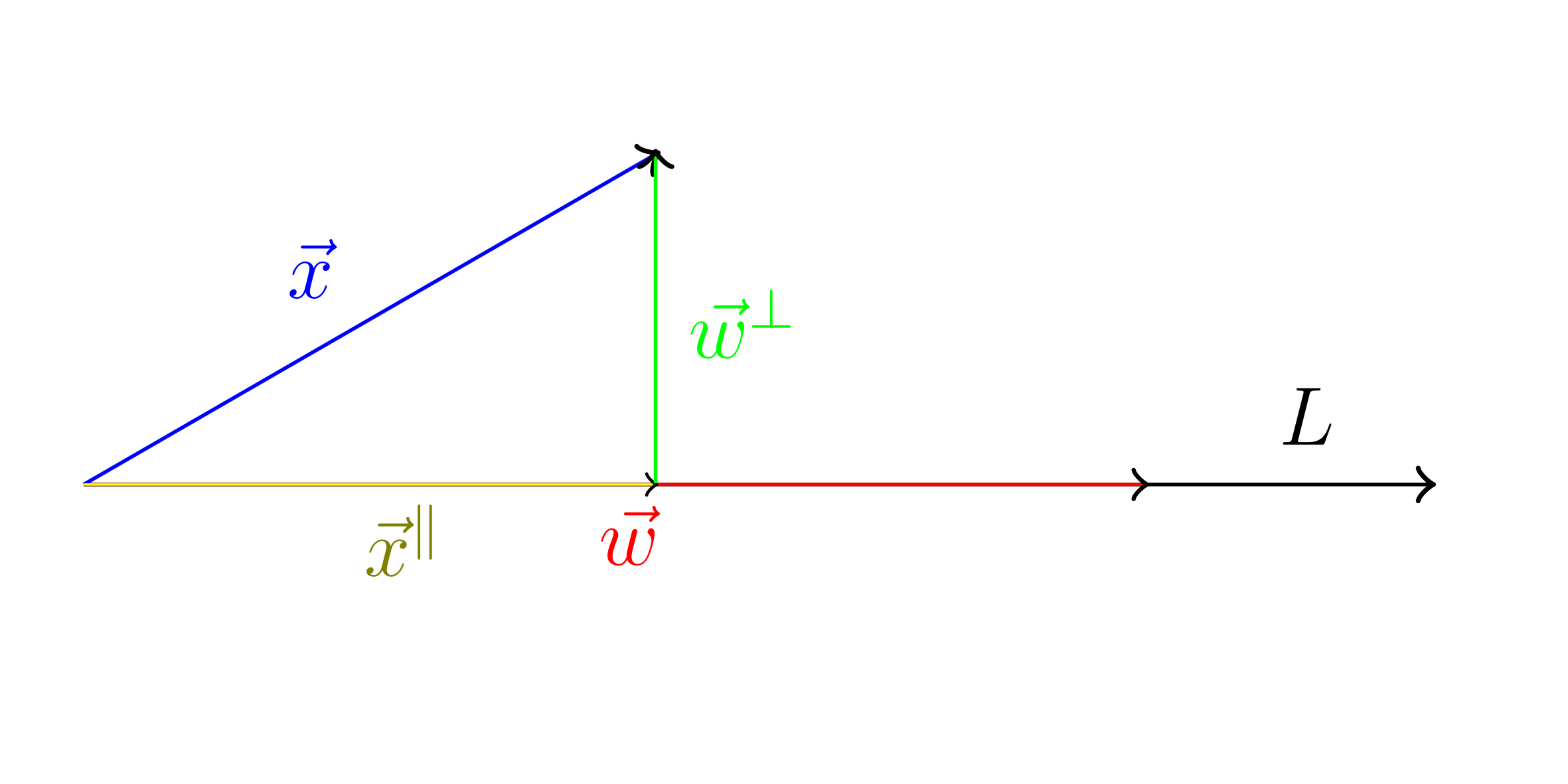
$\vec{x}^{\bot} = \vec{x} - \vec{x}^{\parallel}$:
This is the component of $\vec{x}$ perpendicular to $L$
We want: $\vec{x}^{\parallel} = k \vec{w}$. Find $k$. We also want:
- $\vec{x}^{\bot} \cdot \vec{w} = 0$
$\left( \vec{x} - \vec{x}^{\parallel} \right) \cdot \vec{w} = 0$
$\left( \vec{x} - k \vec{w}\right) \cdot \vec{w} = 0$
$\vec{x} \cdot \vec{w} - k \left( \vec{w} \cdot \vec{w} \right) = 0$
$\vec{x} \cdot \vec{w} = k \left( \vec{w} \cdot \vec{w} \right)$
$k = \frac{\vec{x} \cdot \vec{w}}{\vec{w} \cdot \vec{w}}$
The definition of a projection onto a line:
$\text{proj}_{L} \vec{x} = \frac{\vec{x} \cdot \vec{w}}{\vec{w} \cdot \vec{w}} \vec{w}$
Example
Let $L$ be the line in $\mathbb{R}^{3}$ spanned by $\vec{w} = \begin{bmatrix} 1 \\ 0 \\ -2 \end{bmatrix}$.
Find the orthogonal projection of $\vec{x} = \begin{bmatrix} 2 \\ 1 \\ -1 \end{bmatrix}$ onto $L$ and decompose $\vec{x}$ into $\vec{x}^{\parallel}$ into $\vec{x}^{\parallel} + \vec{x}^{\bot}$.
$\vec{x} \cdot \vec{w} = 2(1) + 0 + (-2)(-1) = 4$
$\vec{w} \cdot \vec{w} = 1(1) + 0(-2)(-2) = 5$
$\vec{x}^{\parallel} = \text{proj}_{L} \vec{x} = \left( \frac{\vec{x} \cdot \vec{w}}{\vec{w} \cdot \vec{w}} \right) \vec{w}$
$\vec{x}^{\parallel} = \frac{4}{5} \begin{bmatrix} 1 \\ 0 \\ 2 \end{bmatrix} = \begin{bmatrix} \frac{4}{5} \\ 0 \\ -\frac{8}{5} \end{bmatrix}$
$\vec{x}^{\bot} = \vec{x} - \vec{x}^{\parallel} = \begin{bmatrix} 2 \\ 1 \\ -1 \end{bmatrix} - \begin{bmatrix} \frac{4}{5} \\ 0 \\ -\frac{8}{5} \end{bmatrix} = \begin{bmatrix} \frac{6}{5} \\ 1 \\ \frac{3}{5} \end{bmatrix}$
Check:
$\vec{x}^{\bot} \cdot \vec{w} = 0 = \begin{bmatrix} \frac{6}{5} \\ 1 \\ \frac{3}{5} \end{bmatrix} \cdot \begin{bmatrix} 1 \\ 0 \\ -2 \end{bmatrix} = \frac{6}{5} - \frac{6}{5} = 0$
Linear transformations $T : \mathbb{R}^{2} \to \mathbb{R}^{2}$ and geometry:
Suppose $\vec{w} = \begin{bmatrix} w_1 \\ w_2 \end{bmatrix}$ is a nonzero vector in $\mathbb{R}^{n}$ and $L = \text{span}\{\vec{w}\}$.
For $\vec{x}$ in $\mathbb{R}^{2}$, the map $\vec{x} \to \text{proj}_{L}\left( \vec{x} \right)$ is a linear transformation!
Let’s find the $2 \times 2$ matrix of orthogonal projection.
$\text{proj} _{L} \left( \vec{e} _{1} \right) = \left( \frac{\vec{e} _{1}\cdot \vec{w}}{\vec{w} \cdot \vec{w}} \right) \vec{w} = \frac{w _{1}}{w _{1}^{2} + w _{2}^{2}} \begin{bmatrix} w _1 \\ w _2 \end{bmatrix}$
$\text{proj} _{L} \left( \vec{e} _{2} \right) = \left( \frac{\vec{e} _{2}\cdot \vec{w}}{\vec{w} \cdot \vec{w}} \right) \vec{w} = \frac{w _{2}}{w _{1}^{2} + w _{2}^{2}} \begin{bmatrix} w _1 \\ w _2 \end{bmatrix}$
Matrix: $\frac{1}{w_1^{2} + w_2^{2}} \begin{bmatrix} w_1^{2} & w_1w_2 \\ w_1w_2 & w_2 ^{2} \end{bmatrix}$
Comment: if $w=\text{span} \{ \begin{bmatrix} u_1 \\ u_2 \end{bmatrix} \}$ where $\begin{bmatrix} u_{1} \\ u_2 \end{bmatrix}$ is unit. i.e. $u_1^{2} + u_2^{2} = 1$
Let’s verify $T$ is a linear transformation. Let $\begin{bmatrix} x_1 \\ x_2 \end{bmatrix}$. Show $\text{proj}_{L} \vec{x} = A \vec{x}$
$\frac{1}{w_1^{2} + w_2^{2}} \begin{bmatrix} w_1^{2} & w_1w_2 \\ w_1w_2 & w_2 ^{2} \end{bmatrix} \begin{bmatrix} x_1 \\ x_2 \end{bmatrix} = \frac{1}{w_1 ^{2} + w_2 ^{2}} \begin{bmatrix} w_1^{2}x_1 + w_1w_2x_2 \\ w_1w_2x_1 + w_2^{2}x_2 \end{bmatrix}$
$= \frac{1}{w_1^{2} + w_2^{2}} \begin{bmatrix} w_1 \left( w_1x_1 + w_2x_2 \right) \\ w_2 \left( w_1x_1 + w_2x_2 \right) \end{bmatrix} = \frac{\vec{w} \cdot \vec{x}}{\vec{v} \cdot \vec{w}} \begin{bmatrix} w_1 \\ w_2 \end{bmatrix}$
Example
Find the matrix of orthogonal projection onto the line spanned by $\vec{w} = \begin{bmatrix} -1 \\ 2 \end{bmatrix}$.
$\frac{1}{\left( -1 \right) ^{2} + 2^{2}} \begin{bmatrix} \left( -1 \right) ^{2} & -2 \\ -2 & 2^{2} \end{bmatrix} = \frac{1}{5} \begin{bmatrix} 1 & -2 \\ -2 & 4 \end{bmatrix} = \begin{bmatrix} \frac{1}{5} & -\frac{2}{5} \\ -\frac{2}{5} & \frac{4}{5} \end{bmatrix}$
Example
Find the matrix of orthogonal projection onto the line $y=x$.
$\text{span}\{ \begin{bmatrix} 1 \\ 1 \end{bmatrix} \}$
$\frac{1}{1^{2} + 1^{2}} \begin{bmatrix} 1^{1} & 1\cdot 1 \\ 1\cdot 1 & 1^{2} \end{bmatrix} = \begin{bmatrix} \frac{1}{2} & \frac{1}{2} \\ \frac{1}{2} & \frac{1}{2} \end{bmatrix}$
Reflection: Let $L = \text{span} \{ \vec{w} \}$ by a line in $\mathbb{R} ^2$.
We use $\vec{x}^{\bot} = \vec{x} - \text{proj}_L (\vec{x})$
$\text{ref} _{L} = \text{proj} _{L}\left( \vec{x} \right) - \vec{x}^{\bot}$
$= \text{proj} _{L} \left( \vec{x} \right) - \left( \vec{x} - \text{proj} _{L}\left( x \right) \right) $
$= 2 \text{proj}_{L} \left( \vec{x} \right) - \vec{x}$
The matrix of reflection about line $L$:
Two ways to compute:
1) Suppose $L = \text{span}\{ \begin{bmatrix} u_1 \\ u_2 \end{bmatrix} \}$, where $u_1 ^{2} + u_2 ^{2} = 1$
$\text{ref} _{L}\left( \vec{x} \right) = 2 \text{proj} _{L} \left( \vec{x} \right) - \vec{x} \to 2 \begin{bmatrix} u _1^{2} & u _1u _2 \\ u _1u _2 & u _2^{2} \end{bmatrix} - I _2 = \begin{bmatrix} 2u _1^{2}-I & 2u _1u _2 \\ 2u _1u _2 & 2u _2^{2} - 1 \end{bmatrix}$
2) The matrix has the form $\begin{bmatrix} a & b \\ b & -a \end{bmatrix}$ where $a^{2} + b^{2} = 1$ and $\begin{bmatrix} a \\ b \end{bmatrix} = \text{ref}_{L}\left( \vec{e}_1 \right) $
Example
Calculate the matrix $\begin{bmatrix} 0 & 1 \\ 1 & 0 \end{bmatrix}$ that yields reflection about the line $y=x$.
$2 \text{proj}_{L}\left( \vec{x} \right) - \vec{x}$
$2 \begin{bmatrix} \frac{1}{2} & \frac{1}{2} \\ \frac{1}{2} & \frac{1}{2} \end{bmatrix} - \begin{bmatrix} 1 & 0 \\ 0 & 1 \end{bmatrix} = \begin{bmatrix} 1-1 & 1 \\ 1 & 1-1 \end{bmatrix} = \begin{bmatrix} 0 & 1 \\ 1 & 0 \end{bmatrix}$
Example
Let $L$ by the $y$-axis, i.e. $L = \text{span}\{ \begin{bmatrix} 0 \\ 1 \end{bmatrix} \}$.
Find $\text{ref}_{L}\left( \vec{e}_1 \right)$ and the matrix of reflection about the line $L$.
$\text{ref}_{L} \left( \vec{e}_1 \right) = \begin{bmatrix} a \\ b \end{bmatrix}$
Matrix: $\begin{bmatrix} a & b \\ b & -a \end{bmatrix}$
$\text{ref} _{L}\left( \vec{e} _{1} \right) = 2 \text{proj} _{L} \left( \vec{e} _1 \right) - \vec{e} _1$
$= 2 \left( \frac{\vec{e}_1 \cdot \vec{e}_2}{\vec{e}_2 \cdot \vec{e}_2} \right) \vec{e}_2 - \vec{e}_1 = 2 \left( \frac{0}{1} \right) \vec{e}_2 - \vec{e}_1 = \begin{bmatrix} -1 \\ 0 \end{bmatrix}$
$A = \begin{bmatrix} -1 & 0 \\ 0 & 1 \end{bmatrix}$
Scaling
For $k > 0,\ T(\vec{x}) = k \vec{x}$.
\[\begin{bmatrix} k & 0 \\ 0 & k \end{bmatrix}\]- $k > 1$ : Dilation
- $0 < k < 1$ : Contraction
Question: Can we interpret the transformation $T(\vec{x}) = \begin{bmatrix} 0 & -1 \\ 1 & 0 \end{bmatrix} \vec{x}$ geometrically?
Answer: Rotation counterclockwise by $\frac{\pi}{2}$ or 90 degrees.
Rotation
Counterclockwise by angle $\theta$.
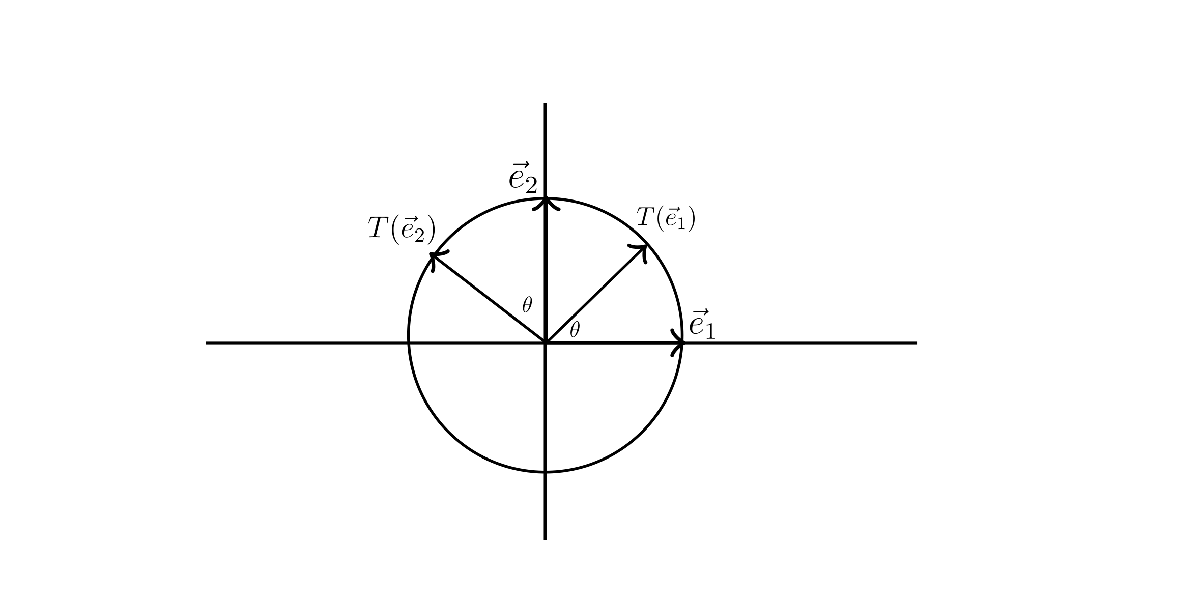
$T\left( \vec{e}_1 \right) = \begin{bmatrix} \cos \theta \\ \sin \theta \end{bmatrix}$
$T\left( \vec{e}_2 \right) = \begin{bmatrix} \cos \left( \theta + \frac{\pi}{2} \right) \\ \sin \left( \theta + \frac{\pi}{2} \right) \end{bmatrix} = \begin{bmatrix} -\sin \theta \\ \cos \theta \end{bmatrix} $
$\therefore A = \begin{bmatrix} \cos \theta & - \sin \theta \\ \sin \theta & \cos \theta \end{bmatrix}$
Transformation Recap:
| Transformation | Matrix |
|---|---|
| Scaling (by $k$) | $kI_2 = \begin{bmatrix} k & 0 \\ 0 & k \end{bmatrix} $ |
| Orthogonal projection onto line $L$ | $\begin{bmatrix} u_1^2 & u_1u_2 \\ u_1u_2 & u_2^2 \end{bmatrix} $, where $\begin{bmatrix} u_1 \\ u_2 \end{bmatrix}$ is a unit vector parallel to $L$ |
| Reflection about a line | $\begin{bmatrix} a & b \\ b & -a \end{bmatrix}$, where $a^2 + b^2 = 1$ |
| Rotation through angle $\theta$ | $\begin{bmatrix} \cos \theta & - \sin \theta \\ \sin \theta & \cos \theta \end{bmatrix}$ or $\begin{bmatrix} a & -b \\ b & a \end{bmatrix} $, where $a^2 + b^2 = 1$ |
| Rotation through angle $\theta$ combined with scaling by $r$ | $\begin{bmatrix} a & -b \\ b & a \end{bmatrix} = r \begin{bmatrix} \cos \theta & - \sin \theta \\ \sin \theta & \cos \theta \end{bmatrix}$ |
| Horizontal shear | $\begin{bmatrix} 1 & k \\ 0 & 1 \end{bmatrix} $ |
| Vertical shear | $\begin{bmatrix} 1 & 0 \ k & 1 \end{bmatrix} $ |
2.3 Matrix Products
Rotation combined with scaling. Suppose
- $T_1 \mathbb{R}^2 \to \mathbb{R}^2$ gives rotation counter clockwise by angle $\theta$
- $T_2 \mathbb{R}^2 \to \mathbb{R}^2$ Scales by $k > 0$
This is in the form $T_2 (T_1(\vec{x}))$
\[T_2 T_1 : \mathbb{R}^2 \to \mathbb{R}^2 \text{ function composition}\] \[(T_2 T_1)(\vec{x}) = k \begin{bmatrix} \cos \theta & - \sin \theta \\ \sin \theta & \cos \theta \end{bmatrix} \vec{x}\]What is the matrix?
\[\begin{bmatrix} k\cos \theta & -k \sin \theta \\ k \sin \theta & k \cos \theta \end{bmatrix} = \begin{bmatrix} k & 0 \\ 0 & k \end{bmatrix} \begin{bmatrix} \cos \theta & -\sin \theta \\ \sin \theta & \cos \theta \end{bmatrix}\] \[\text{Composition of Transformations} \leftrightarrow \text{Matrix Product}\]The matrix product BA: Suppose $B$ is an $n\times p$ matrix and $A$ is a $p \times m$ matrix.
Size of $BA$: $[n \times p] [p\times m] \to n\times m$
Columns of the product $BA$: Suppose $A = \begin{bmatrix} | & | & & | \\ \vec{v}_1 & \vec{v}_2 & \cdots & \vec{v}_m \\ | & | & & | \end{bmatrix}$
\[BA = \begin{bmatrix} | & | & & | \\ B\vec{v}_1 & B\vec{v}_2 & \cdots & B\vec{v}_m \\ | & | & & | \\ \end{bmatrix}\]Entries of $BA$ are dot products.
(i, j) - entry of BA = [row i of B] * [Column j of A]
Example
\[\begin{bmatrix}
1 & 3 & -1 \\
2 & 0 & 1
\end{bmatrix}
\begin{bmatrix}
1 & 3 \\
2 & 0 \\
0 & -1
\end{bmatrix}
=
\begin{bmatrix}
7 & 4 \\
2 & 5
\end{bmatrix}\]
Rows of the product $BA$ [ith row of BA] = [ith row of B] A
Example
\[\begin{bmatrix}
2 & 0 & 1
\end{bmatrix}
\begin{bmatrix}
1 & 3 \\
2 & 0 \\
0 & -1
\end{bmatrix}
=
\begin{bmatrix}
2 & 5
\end{bmatrix}\]
Example
Suppose $A = \begin{bmatrix} 5 & 3 & 2 & 0 \end{bmatrix}$ and $B = \begin{bmatrix} 1 \\ -1 \\ 2 \\ -3 \end{bmatrix}$. Find $AB$ and $BA$.
\[AB = 5 - 3 + 4 + 0 = \begin{bmatrix} 6 \end{bmatrix}\] \[BA = \begin{bmatrix} 1 \\ -1 \\ 2 \\ -3 \end{bmatrix} \begin{bmatrix} 5 & 3 & 2 & 0 \end{bmatrix} = \begin{bmatrix} 5 & 3 & 2 & 0 \\ -5 & -3 & -2 & 0 \\ 10 & 6 & 4 & 0 \\ -15 & -9 & -6 & 0 \end{bmatrix}\]Notice by these examples that $AB \neq BA$ (they are not even the same size).
Example
Let $A = \begin{bmatrix} 2 & 1 \\ -3 & 0 \end{bmatrix}$, $B = \begin{bmatrix} 1 & 0 \\ 1 & 0 \end{bmatrix}$, and $C = \begin{bmatrix} 0 & 1 \\ -1 & 0 \end{bmatrix}$. Show that $A(B+C) = AB + AC$
\[\begin{bmatrix} 2 & 1 \\ -3 & 0 \end{bmatrix} \left( \begin{bmatrix} 1 & 0 \\ 1 & 0 \end{bmatrix} + \begin{bmatrix} 0 & 1 \\ -1 & 0 \end{bmatrix} \right) = \begin{bmatrix} 2 & 1 \\ -3 & 0 \end{bmatrix} \begin{bmatrix} 1 & 1 \\ 0 & 0 \end{bmatrix} = \begin{bmatrix} 2 & 2 \\ -3 & -3 \end{bmatrix}\]Properties
- $A(B+C) = AB + AC$ and $(C+D)A = CA + DA$
- $I_nA = AI_m = A$
- $K(AB) = (KA)B = A(KB)$
- $A(BC) = (AB)C$
Be Careful!
- $AB \neq BA$ generally even if they are the same size
- If $AB = AC$, it does not generally follow that $B=C$
- If $AB=0$, it does not generally follow that $A=0$ or $B=0$
Example
\[\begin{bmatrix} 1 & 0 \\ 1 & 0 \end{bmatrix} \begin{bmatrix} 4 & 1 \\ 1 & 1 \end{bmatrix} =
\begin{bmatrix} 4 & 1 \\ 4 & 1 \end{bmatrix}\]
and
\[\begin{bmatrix} 1 & 0 \\ 1 & 0 \end{bmatrix} \begin{bmatrix} 4 & 1 \\ -1 & 2 \end{bmatrix} = \begin{bmatrix} 4 & 1 \\ 4 & 1 \end{bmatrix}\]
Example
\[\begin{bmatrix} 4 & 1 \\ 1 & 1 \end{bmatrix} \begin{bmatrix} 1 & 0 \\ 1 & 0 \end{bmatrix} = \begin{bmatrix} 5 & 0 \\ 2 & 0 \end{bmatrix}\]
Example
\[\begin{bmatrix}
2 & 0 \\
0 & 0 \\
-4 & 0
\end{bmatrix}
\begin{bmatrix}
0 & 0 \\
1 & 6
\end{bmatrix}
=
\begin{bmatrix}
0 & 0 \\
0 & 0 \\
0 & 0
\end{bmatrix}\]
Definition: For matrices $A$ and $B$, we say $A$ and $B$ commute provided $AB = BA$. Note that both $A$ and $B$ must be $n \times n$.
- We see $\begin{bmatrix} 1 & 0 \\ 1 & 0 \end{bmatrix}$ an $\begin{bmatrix} 4 & 1 \\ 1 & 1 \end{bmatrix}$ do not commute.
- $I_n$ commutes with any $n \times n$ matrix
Example
\[\begin{bmatrix} a & b \\ c & d \end{bmatrix} \begin{bmatrix} 1 & 0 \\ 1 & 0 \end{bmatrix} =
\begin{bmatrix} a + b & 0 \\ c+d & 0 \end{bmatrix}\]
\[\begin{bmatrix} 1 & 0 \\ 1 & 0 \end{bmatrix} \begin{bmatrix} a & b \\ c & d \end{bmatrix} =
\begin{bmatrix} a & b \\ a & b \end{bmatrix}\]
$a+b = a$
$c+d = a$
$b = 0$
$b=0$
\[\begin{bmatrix} c+d & 0 \\ c & d \end{bmatrix}\]
Example
Find all matrices that commute with $\begin{bmatrix} 2 & 0 & 0 \\ 0 & 3 & 0 \\ 0 & 0 & 4 \end{bmatrix} $
\[\begin{bmatrix} 2 & 0 & 0 \\ 0 & 3 & 0 \\ 0 & 0 & 4 \end{bmatrix} \begin{bmatrix} a & b & c \\ d & e & f \\ g & h & i \end{bmatrix} = \begin{bmatrix} 2a & 2b & 2c \\ 3d & 3e & 3f \\ 4g & 4h & 4i \end{bmatrix}\] \[\begin{bmatrix} a & b & c \\ d & e & f \\ g & h & i \end{bmatrix} \begin{bmatrix} 2 & 0 & 0 \\ 0 & 3 & 0 \\ 0 & 0 & 4 \end{bmatrix} = \begin{bmatrix} 2a & 3b & 4c \\ 2d & 3e & 4f \\ 2g & 3h & 4i \end{bmatrix}\]$2b = 3b$
$2c = 4c$
$3d = 2d$
$3f = 4f$
$4g = 2g$
$4h = 3h$
\[\begin{bmatrix} a & 0 & 0 \\ 0 & e & 0 \\ 0 & 0 & i \end{bmatrix}\]Power of a Matrix
Suppose $A$ is $n \times n$. For $k \ge 1$ integer, define the $k$th power of $A$.
\[A^k = \underbrace{AAAA \cdots A}_{k \text{ times}}\]Properties:
- $A^pA^q = A^{p+q}$
- $\left( A^{p} \right)^{q} = A^{pq}$
Example
$A = \begin{bmatrix} 0 & 1 & 2 \\ 0 & 0 & -1 \\ 0 & 0 & 0 \end{bmatrix}$. Find $A^{2}$, $A^{3}$. What is $A^{k}$ for $k > 3$?
\[A^2 = \begin{bmatrix} 0 & 1 & 2 \\ 0 & 0 & -1 \\ 0 & 0 & 0 \end{bmatrix} \begin{bmatrix} 0 & 1 & 2 \\ 0 & 0 & -1 \\ 0 & 0 & 0 \end{bmatrix} = \begin{bmatrix} 0 & 0 & -1 \\ 0 & 0 & 0 \\ 0 & 0 & 0 \end{bmatrix}\] \[A^3 = \begin{bmatrix} 0 & 1 & 2 \\ 0 & 0 & -1 \\ 0 & 0 & 0 \end{bmatrix} \begin{bmatrix} 0 & 0 & -1 \\ 0 & 0 & 0 \\ 0 & 0 & 0 \end{bmatrix} = \begin{bmatrix} 0 & 0 & 0 \\ 0 & 0 & 0 \\ 0 & 0 & 0 \end{bmatrix}\]Note that $A^3 = 0$, but $A \neq 0$.
$\text{rank}\left( A \right) = 2$ $\text{rank}\left( A^{2} \right) = 1$ $\text{rank}\left( A^{3} \right) = 0$
Example
\[\begin{bmatrix}
a & 0 & 0 \\
0 & b & 0 \\
0 & 0 & c
\end{bmatrix}
\begin{bmatrix}
a & 0 & 0 \\
0 & b & 0 \\
0 & 0 & c
\end{bmatrix}
=
\begin{bmatrix}
a^2 & 0 & 0 \\
0 & b^2 & 0 \\
0 & 0 & c^2
\end{bmatrix}\]
Exam 1
Will most likely have a “find all matrices that commute with” question
100 minutes
Practice Quiz 2
1) Compute the product $A \vec{x}$ using paper and pencil: $\begin{bmatrix} 1 & 3 \\ 1 & 4 \\ -1 & 0 \\ 0 & 1 \end{bmatrix} \begin{bmatrix} 1 \\ -2 \end{bmatrix}$.
\[1 \begin{bmatrix} 1 \\ 1 \\ -1 \\ 0 \end{bmatrix} - 2 \begin{bmatrix} 3 \\ 4 \\ 0 \\ 1 \end{bmatrix} = \begin{bmatrix} -5 \\ -7 \\ -1 \\ -2 \end{bmatrix}\]2) Let $A$ be a $6 \times 3$ matrix. We are told that $A \vec{x} = \vec{0}$ has a unique solution.
a) What is the reduced row-echelon form of $A$? b) Can $A\vec{x} = \vec{b}$ be an inconsistent system for some $\vec{b} \in \mathbb{R}^6$? Justify your answer. c) Can $A\vec{x} = \vec{b}$ have infinitely many solutions for some $\vec{b} \in \mathbb{R}^6$? Justify your answer.
Solution
a)
\[\begin{bmatrix} 1 & 0 & 0 \\ 0 & 1 & 0 \\ 0 & 0 & 1 \\ 0 & 0 & 0 \\ 0 & 0 & 0 \\ 0 & 0 & 0 \end{bmatrix}\]b) Yes; we can have $\begin{bmatrix} 0 & 0 & 0 & \big| & c \end{bmatrix}$ where $c\neq 0$ in $\text{ref}\begin{bmatrix} a & \big| & \vec{b} \end{bmatrix}$.
c) No; there are no free variables
3) Let $\vec{w} = \begin{bmatrix} -2 \\ 2 \\ 0 \\ 1 \end{bmatrix}$, $L = \text{span}\left( \vec{w} \right)$, and $\vec{x} = 3 \vec{e}_3 \in \mathbb{R}^4$. Show your work
a) Find $\vec{x}^{\parallel} = \text{proj}_L \left( \vec{x} \right)$, the projection of $\vec{x}$ onto $L$. b) Find $\vec{x}^{\bot}$, the component of $\vec{x}$ orthogonal to $L$.
Solution
a) $\text{proj}_L \left( \vec{x} \right) = \left( \frac{\vec{x} \cdot \vec{w}}{\vec{w} \cdot \vec{w}} \right) \vec{w}$
$\vec{x} \cdot \vec{w} = 0 + 6 + 0 + 0 = 6$
$\vec{w} \cdot \vec{w} = 4 + 4 + 0 + 1 = 9$
$\text{proj}_{L} \left( \vec{x} \right) = \frac{2}{3} \begin{bmatrix} -2 \\ 2 \\ 0 \\ 1 \end{bmatrix} = \begin{bmatrix} -\frac{4}{3} \\ \frac{4}{3} \\ 0 \\ \frac{2}{3} \end{bmatrix}$
b) $\vec{x}^{\bot} = \vec{x} - \text{proj}_L \left( \vec{x} \right)$
$= \begin{bmatrix} 0 \\ 3 \\ 0 \\ 0 \end{bmatrix} - \begin{bmatrix} -\frac{4}{3} \\ \frac{4}{3} \\ 0 \\ \frac{2}{3} \end{bmatrix} = \begin{bmatrix} \frac{4}{3} \\ \frac{5}{3} \\ 0 \\ -\frac{2}{3} \end{bmatrix}$
4) Suppose $T_1 : \mathbb{R}^{2} \to \mathbb{R}^{3}$ is given by $T_1 \left( \begin{bmatrix} x \\ y \end{bmatrix} \right) = \begin{bmatrix} 0 \\ x - y \\ 3y \end{bmatrix}$ and $T_2 : \mathbb{R}^{2} \to \mathbb{R}^{2}$ is a scaling transformation with $T_2 \left( \begin{bmatrix} 1 \\ 7 \end{bmatrix} \right) = \begin{bmatrix} 3 \\ 21 \end{bmatrix}$. Show your work
a) Find the matrix of the transformation $T_1$. b) Find the matrix of the transformation $T_2$.
Solution
a) $\begin{bmatrix} | & | \\ T\left( \vec{e}_1 \right) & T\left( \vec{e}_2 \right) \\ | & | \end{bmatrix}$
$T \begin{bmatrix} 1 \\ 0 \end{bmatrix} = \begin{bmatrix} 0 \\ 1 \\ 0 \end{bmatrix}$, $T \begin{bmatrix} 0 \\ 1 \end{bmatrix} = \begin{bmatrix} 0 \\ -1 \\ 3 \end{bmatrix}$
$A = \begin{bmatrix} 0 & 0 \\ 1 & -1 \\ 0 & 3 \end{bmatrix}$
b) Scaling by $k=3$
$\begin{bmatrix} 3 & 0 \\ 0 & 3 \end{bmatrix}$
5) Let $T : \mathbb{R}^{2} \to \mathbb{R}^{3}$ be a linear transformation such that $T \left( 2 \vec{e}_1 \right) = \begin{bmatrix} 2 \\ 2 \\ 2 \end{bmatrix}$ and $T \left( \vec{e}_1 + \vec{e}_2 \right) = \begin{bmatrix} 2 \\ 3 \\ 4 \end{bmatrix}$. Find $T \left( \vec{e}_1 \right)$ and $T \left( \vec{e}_2 \right)$. Show your work.
$T \left( 2 \vec{e}_1 \right) = 2 T \left( \vec{e}_1 \right) = \begin{bmatrix} 2 \\ 2 \\ 2 \end{bmatrix}$
$T \left( \vec{e}_1 \right) = \begin{bmatrix} 1 \\ 1 \\ 1 \end{bmatrix}$
$T \left( \vec{e}_1 + \vec{e}_2 \right) = T \left( \vec{e}_1 \right) + T \left( \vec{e}_2 \right) = \begin{bmatrix} 2 \\ 3 \\ 4 \end{bmatrix}$
$T \left( \vec{e}_2 \right) = \begin{bmatrix} 2 \\ 3 \\ 4 \end{bmatrix} - T \left( \vec{e}_1 \right) = \begin{bmatrix} 1 \\ 2 \\3 \end{bmatrix}$
2.4 Inverse of a Linear Transformation
In Math1365 (or other courses), you see diagrams for $f : X \to Y$ function.
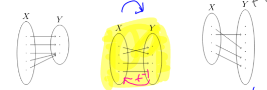
Definition:
We say the function $f : X \to Y$ is invertible provided for each $y$ in $Y$, there is a unique $x$ in $X$ with $f(x) = y$ if any only if $f^{-1} : Y \to X$ is a function $f^{-1}(y) = x$ provided $f(x) = y$.
Same notation for linear transformation $T : \mathbb{R}^{n} \to \mathbb{R}^{n}$
A square $n \times n$ matrix $A$ is invertible provided the map $T \left( \vec{x} \right) = A \vec{x}$ is invertible. The matrix for $T^{-1}$ is denoted $A^{-1}$.
Note:
- $T T^{-1} (\vec{y}) = \vec{y}$ for any $\vec{y}$ in $\mathbb{R}^{n}$
- $T^{-1}T(\vec{x}) = \vec{x}$ for any $\vec{x}$ in $\mathbb{R}^{n}$
- $AA^{-1} = I_{n}$ and $A^{-1}A = I_{n}$
$A$ invertible means $A\vec{x} = \vec{b}$ has a unique solution for every $\vec{b}$ in $\mathbb{R}^{n}$.
- The unique solution is $\vec{x} = A^{-1}\vec{b}$
For our discussion of rank: $A$ is invertible is equivalent to…
- $\text{rank}(A) = n$
- $\text{rref}(A) = I_n$
- The only solution to $A\vec{x} = \vec{0}$ is $\vec{x} = \vec{0}$
How to find $A^{-1}$ if $A$ is $n \times n$,
- Form the $n \times \left( 2n \right)$ matrix $\begin{bmatrix} A & \big| & I \end{bmatrix}$
- Perform elementary row operations to find $\text{rref} \begin{bmatrix} A & \big| & I \end{bmatrix}$
Then,
- If $\text{rref} \begin{bmatrix} A & \big| & I \end{bmatrix} = \begin{bmatrix} I & \big| & B\end{bmatrix}$ then $B = A^{-1}$.
- If $\text{rref} \begin{bmatrix} A & \big| & I \end{bmatrix}$ is not of this form then $A$ is not invertible.
Example
$A = \begin{bmatrix} 2 & 3 \\ 1 & 1 \end{bmatrix}$. Find $A^{-1}$.
\[\begin{bmatrix} 2 & 3 & \big| & 1 & 0 \\ 1 & 1 & \big| & 0 & 1 \end{bmatrix} \to \begin{bmatrix} 1 & 1 & \big| & 0 & 1 \\ 2 & 3 & \big| & 1 & 0 \end{bmatrix} \to\] \[\begin{bmatrix} 1 & 1 & \big| & 0 & 1 \\ 0 & 1 \big| & 1 & -2 \end{bmatrix} \to \begin{bmatrix} 1 & 0 & \big| & -1 & 3 \\ 0 & 1 & \big| & 1 & -2 \end{bmatrix}\] \[A^{-1} = \begin{bmatrix} -1 & 3 \\ 1 & -2 \end{bmatrix}\]
Example
$A = \begin{bmatrix} 2 & 2 \ 1 & 1 \end{bmatrix}$. Find $A^{-1}$.
\[\begin{bmatrix} 2 & 2 & \big| & 1 & 0 \end{bmatrix} \to \begin{bmatrix} 1 & 1 & \big| & 0 & 1 \end{bmatrix} \to \begin{bmatrix} 1 & 1 & \big| & 0 & 1 \\ 0 & 0 & \big| & 1 & -2 \end{bmatrix}\]$A$ is not invertible
Example
$A = \begin{bmatrix} 1 & 3 & 1 \\ 1 & 4 & 1 \\ 2 & 0 & 1 \end{bmatrix}$. Find $A^{-1}$.
\[\begin{bmatrix} 2 & 2 & \big| & 1 & 0 \\ 1 & 1 & \big| & 0 & 1 \\ \end{bmatrix} \to \begin{bmatrix} 1 & 3 & 1 & \big| & 1 & 0 & 0 \\ 0 & 1 & 0 & \big| & -1 & 1 & 0 \\ 0 & -6 & -1 & \big| & -2 & 0 & 1 \end{bmatrix}\] \[\to \begin{bmatrix} 1 & 3 & 1 & \big| & 1 & 0 & 0 \\ 0 & 1 & 0 & \big| & -1 & 1 & 0 \\ 0 & 0 & -1 & \big| & -8 & 6 & 1 \end{bmatrix}\] \[\to \begin{bmatrix} 1 & 3 & 1 & \big| & 1 & 0 & 0 \\ 0 & 1 & 0 & \big| & -1 & 1 & 0 \\ 0 & 0 & 1 & \big| & 8 & -6 & -1 \end{bmatrix} \to \begin{bmatrix} 1 & 3 & 0 & \big| & -7 & 6 & 1\\ 0 & 1 & 0 & \big| & -1 & 1 & 0 \\ 0 & 0 & 1 & \big| & 8 & -6 & -1 \end{bmatrix}\] \[\to \begin{bmatrix} 1 & 0 & 0 & \big| & -4 & 3 & 1 \\ 0 & 1 & 0 & \big| & -1 & 1 & 0 \\ 0 & 0 & 1 & \big| & 8 & -6 & -1 \end{bmatrix}\] \[A^{-1} = \begin{bmatrix} -4 & 3 & 1 \\ -1 & 1 & 0 \\ 8 & -6 & -1 \end{bmatrix}\]
Example
Find all solutions to the system $A\vec{x} = \vec{b}$ where $A = \begin{bmatrix} 1 & 3 & 1 \\ 1 & 4 & 1 \\ 2 & 0 & 1 \end{bmatrix}$ and $\vec{b} = \begin{bmatrix} 1 \\ -1 \\ 0 \end{bmatrix}$
\[A^{-1} = \begin{bmatrix} -4 & 3 & 1 \\ -1 & 1 & 0 \\ 8 & -6 & -1 \end{bmatrix}\] \[\vec{x} = A^{-1}\vec{b} = \begin{bmatrix} -4 & 3 & 1 \\ -1 & 1 & 0 \\ 8 & -6 & -1 \end{bmatrix} \begin{bmatrix} 1 \\ -1 \\ 0 \end{bmatrix} = \begin{bmatrix} -7 \\ -2 \\ 14 \end{bmatrix}\]Theorem:
Let $A$, $B$ be $n \times n$ matrices with $BA = I_n$ then,
- $A$, $B$ are both invertible
- $A^{-1} = B$ and $B^{-1} = A$
- $AB = I_n$
Proof of 1) Assume $A$, $B$ are $n\times n$ matrices with $BA = I_n$. Suppose $A\vec{x} = \vec{0}$. Show $\vec{x}=0$. Multiply by $B$: $BA\vec{x} = B\vec{0}$ rewriting $I\vec{x} = \vec{0}$ meaning $\vec{x} = \vec{0}$. Thus, $A$ is invertible. Then, $BA A^{-1} = IA^{-1}$ and $B = A^{-1}$. $B$ is invertible.
Using the theorem:
If $A$, $B$ are $n\times n$ invertible matrices then so is $BA$ and $\left( BA \right) ^{-1} = A^{-1}B^{-1}$.
Proof: $\left( BA \right) \left( A^{-1}B^{-1} \right) = B\left( A A^{-1} \right) B^{-1} = BIB^{-1} = B B^{-1} = I$.
Exercise: Suppose $A$ is an $n\times n$ invertible matrix.
Is $A^{2}$ invertible? If so, what is $\left( A^{-2} \right) ^{-1}$?
Yes; $A^{-1}A^{-1} = \left( A^{-1} \right) ^{2}$
Is $A^{3}$ invertible? If so, what is $\left( A^{3} \right)^{-1}$?
Yes; $\left( A^{-1} \right) ^{3}$
$\left( A AA \right) \left( A^{-1}A^{-1}A^{-1} \right) = A A A^{-1}A^{-1} = A A^{-1} = I$
Back to $2\times 2$ matrices: We saw
- For $A = \begin{bmatrix} 2 & 3 \\ 1 & 1 \end{bmatrix}$, $A^{-1} = \begin{bmatrix} -1 & 3 \\ 1 & -2 \end{bmatrix}$.
- The matrix $\begin{bmatrix} 2 & 2 \\ 1 & 1 \end{bmatrix}$ is not invertible
Theorem: Consider a $2\times 2$ matrix $A = \begin{bmatrix} a & b \\ c & d \end{bmatrix}$.
$A$ is invertible if and only if $ad - bc \neq 0$
If $A$ is invertible, then $A^{-1}$ = $\frac{1}{ad-bc} \begin{bmatrix} d & -b \\ -c & a \end{bmatrix}$
The number $ad - bc$ is a determinant of $A = \begin{bmatrix} a & b \\ c& d \end{bmatrix}$.
Example
$A = \begin{bmatrix} 4 & 7 \\ 0 & 1 \end{bmatrix}$. Find $\text{det}(A)$ and $A^{-1}$.
$\text{det}(A) = 4 - 0 = 4$
$A^{-1} = \frac{1}{4} \begin{bmatrix} 1 & -7 \\ 0 & 4 \end{bmatrix}$
3.1 Image and Kernel of a Linear Transformation
Definition:
Let $T : \mathbb{R}^{m} \to \mathbb{R}^{n}$ be a linear transformation.
The Image of $T$, denoted $\text{im}\left( T \right)$ : $\text{im}\left( T \right) = \{T \left( \vec{x} \right) : x \in \mathbb{R}^{m} \} \subseteq \mathbb{R}^{n}$
The kernel of $T$ $\text{ker}\left( T \right)$ : $\text{ker}\left( T \right) = \{ \vec{x} \in \mathbb{R}^{m} : T \left( \vec{x} \right) = \vec{0} \} \subseteq \mathbb{R}^{m}$
Example
What is $\text{ker} \left( T \right)$ and $\text{im}\left( T \right)$ when $T : \mathbb{R}^{2} \to \mathbb{R}^{2}$ is
1) Projection onto the line $y = -x$. 2) Reflection about the line $y = -x$.
Solution
1)
$\vec{w} = \begin{bmatrix} -1 \\ 1 \end{bmatrix}$
$L = \text{span}\left( \begin{bmatrix} -1 \\ 1 \end{bmatrix} \right) $
$\text{proj}_{L} \left( \vec{x} \right) = \left( \frac{\vec{w} \cdot \vec{w}}{\vec{w} \cdot \vec{w}} \right) \vec{w}$
$\vec{x}$ is in $\text{ker}\left( T \right)$ provided $\vec{x} \cdot \begin{bmatrix} -1 \\ 1 \end{bmatrix} = \vec{0}$
$\text{ker}\left( T \right) = \{ \begin{bmatrix} x_1 \\ x_2 \end{bmatrix} : -x_1 + x_2 = 0 \}$
$\text{im}\left( T \right) = L$
2) $\text{ker}\left( T \right) = \{ \vec{0} \}$
$\text{im}\left( T \right) = \mathbb{R}^{2}$
Suppose $T : \mathbb{R}^{m} \to \mathbb{R}^{n}$ is a linear transformation. There is an $n \times m$ matrix $A = \begin{bmatrix} | & | & & | \\ \vec{a}_1 & \vec{a}_2 & \cdots & \vec{a}_m \\ | & | & & | \end{bmatrix}$ such that $T \left( \vec{x} \right) = A \vec{x}$ for all $\vec{x}$ in $\mathbb{R}^{m}$.
Image of $T$ (Also written $\text{im}\left( A \right)$):
$\text{im}\left( T \right) = \{ A\vec{x} : \vec{x} \in \mathbb{R}^{m} = \{ x_1\vec{a}_1 + x_2\vec{a}_2 + \cdots + x_m\vec{a}_m : x_i \in \mathbb{R} = \{ \text{all linear combinations of } \vec{a}_1,\ \vec{a}_2,\ \cdots ,\ \vec{a}_m \} = \text{span}\left( \vec{a}_1,\ \vec{a}_2,\ \cdots, \vec{a}_m \right)$
Kernel of $T$ (Also written $\text{ker}\left( A \right)$:
$\text{ker}\left( T \right) = \{ x \in \mathbb{R}^{m} : A\vec{x} = \vec{0} \} = \{ \text{all solutions to } A\vec{x} = \vec{0} \}$
Example
Find vectors that span the kernel of $\begin{bmatrix} 1 & -3 \\ -3 & 9 \end{bmatrix}$.
\[\begin{bmatrix} 1 & -3 & \big| & 0 \\ -3 & 9 & \big| & 0 \end{bmatrix} \to \begin{bmatrix} 1 & -3 & \big| & 0 \\ 0 & 0 & \big| & 0 \end{bmatrix}\]$x_2 = t$
$x_1 - 3t = 0$
$x_1 = 3t$
$\begin{bmatrix} 3t \\ t \end{bmatrix} = t \begin{bmatrix} 3 \\ 1 \end{bmatrix}$
$\text{ker}\left( A \right) = \text{span} \{ \begin{bmatrix} 3 \\ 1 \end{bmatrix} \}$
Example
Find vectors that span the kernel of $\begin{bmatrix} 1 & 3 & 0 & 5 \\ 2 & 6 & 1 & 16 \\ 5 & 15 & 0 & 25 \end{bmatrix}$.
\[\begin{bmatrix} 1 & 3 & 0 & 5 \\ 2 & 6 & 1 & 16 \\ 5 & 15 & 0 & 25 \end{bmatrix} \to \begin{bmatrix} 1 & 3 & 0 & 5 \\ 0 & 0 & 1 & 6 \\ 0 & 0 & 0 & 0 \end{bmatrix}\]$x_2 = t$
$x_4 = r$
$x_1 = -3t - 5r$
$x_3 = -6r$
\[\begin{bmatrix} -3t - 5t \\ t \\ -6r \\ r \end{bmatrix} = t \begin{bmatrix} -3 \\ 1 \\ 0 \\ 0 \end{bmatrix} + r \begin{bmatrix} -5 \\ 0 \\ -6 \\ 1 \end{bmatrix} = \text{span} \{ \begin{bmatrix} -3 \\ 1 \\ 0 \\ 0 \end{bmatrix}, \begin{bmatrix} -5 \\ 0 \\ -6\\ 1 \end{bmatrix} \}\]
Example
Find vectors that span the kernel of $\begin{bmatrix} 1 & 1 & -2 \\ -1 & -1 & 2 \end{bmatrix}$
\[\begin{bmatrix} 1 & 1 & -2 \\ -1 & -1 & 2 \end{bmatrix} \to \begin{bmatrix} 1 & 1 & -2 \\ 0 & 0 & 0 \end{bmatrix}\]$x_1 = -r + 2s$
$x_2 = r$
$x_3 = s$
\[\begin{bmatrix} -r + 2s \\ r \\ s \end{bmatrix} = r \begin{bmatrix} -1 \\ 1 \\ 0 \end{bmatrix} + s \begin{bmatrix} 2 \\ 0 \\ 1 \end{bmatrix}\] \[\text{ker}(A) = \text{span} \{ \begin{bmatrix} -1 \\ 1 \\ 0 \end{bmatrix}, \begin{bmatrix} 2 \\ 0 \\1 \end{bmatrix} \}\]Properties of the kernel:
- $\vec{0} \in \text{ker}\left( A \right)$
- If $\vec{v}_1$, $\vec{v}_2 \in \text{ker}\left( A \right)$, then $\vec{v}_1 + \vec{v}_2 \in \text{ker}\left( A \right)$. Closed under addition.
- If $\vec{v} \in \text{ker}\left( A \right)$ then $k\vec{v} \in \text{ker}\left( A \right)$. Closed under scaler multiplication
Proof:
- $A\vec{0} = \vec{0}$
- If $A\vec{v}_1 = \vec{0}$ and $A\vec{v}_2 = \vec{0}$, then $A \left( \vec{v}_1 + \vec{v}_2\right) = A\vec{v}_1 + A \vec{v}_2 = \vec{0} + \vec{0} = \vec{0}$
- If $A\vec{v}$, then $A\left( k\vec{v} \right) = kA\vec{v} = k\vec{0} = \vec{0}$.
Give as few vectors as possible!!
Example
$A = \begin{bmatrix} 1 & -3 \\ -3 & 9 \end{bmatrix}$
$\text{rref}(A) = \begin{bmatrix} 1 & -3 \\ 0 & 0 \end{bmatrix}$
$x \begin{bmatrix} 1 \\ -3 \end{bmatrix} + y \begin{bmatrix} -3 \\ 9 \end{bmatrix} = \left( x - 3y \right) \begin{bmatrix} 1 \\ -3 \end{bmatrix}$
$\text{im}(A) = \text{span}\left( \begin{bmatrix} 1 \\ -3 \end{bmatrix} \right)$
Example
$A = \begin{bmatrix} 1 & -1 & 1 & 2 \\ -2 & 2 & 0 & 0 \\ -1 & 1 & 3 & 1 \end{bmatrix}$
$\text{rref}\left( A \right) = \begin{bmatrix} 1 & -1 & 0 & 0 \\ 0 & 0 & 1 & 0 \\ 0 & 0 & 0 & 1 \end{bmatrix}$
$\text{lm}\left( A \right) = \text{span} \{ \begin{bmatrix} 1 \\ -2 \\ -1 \end{bmatrix}, \begin{bmatrix} -1 \\ 2 \\ 1 \end{bmatrix}, \begin{bmatrix} 1 \\ 0 \\ 3 \end{bmatrix}, \begin{bmatrix} 2 \\ 0 \\ 1 \end{bmatrix} \}$
$\text{im}\left( A \right) = \text{span} \{ \begin{bmatrix} 1 \\ -2 \\ -1 \end{bmatrix}, \begin{bmatrix} 1 \\ 0 \\ 3 \end{bmatrix}, \begin{bmatrix} 2 \\ 0 \\ 1 \end{bmatrix} \}$
Careful: Make sure you use columns in $A$ corresponding to leading 1’s in $\text{rref}$.
Example
$A = \begin{bmatrix} 1 & 2 & 3 \\ 1 & 2 & 3 \\ 1 & 2 & 3 \\ 1 & 2 & 3 \end{bmatrix}$
$\text{rref}\left( A \right) = \begin{bmatrix} 1 & 2 & 3 \\ 0 & 0 & 0 \\ 0 & 0 & 0 \\ 0 & 0 & 0 \end{bmatrix}$
$\text{im}\left( A \right) = \text{span}\{ \begin{bmatrix} 1 \\ 1 \\ 1\\ 1 \end{bmatrix} \} \neq \text{span} \{ \begin{bmatrix} 1 \\ 0 \\ 0 \\ 0 \end{bmatrix} \} = \text{im} \left( \text{rref} \left( A \right) \right)$
Note: $\text{im}\left( T \right)$ or $\text{im}\left( A \right)$ is a subspace of $\mathbb{R}^{n}$.
- $\vec{0} \in \text{im}\left( A \right)$ to
- Closed under addition and scaler multiplication
Exercise
$I_3 = \begin{bmatrix} 1 & 0 & 0 \\ 0 & 1 & 0 \\ 0 & 0 & 1 \end{bmatrix}$. What is $\text{ker}\left( I_3 \right)$ and $\text{im}\left( I_3 \right)$?
$\text{ker}\left( I_3 \right) = \{ \vec{0} \}$
$\text{im}\left( I_3 \right) = \mathbb{R}^{3}$
Generally, if $A$ is $n\times n$ matrix,
$\text{im}\left( A \right) = \mathbb{R}^{n}$ if and only if $\text{ker}\left( A \right) = \{ \vec{0} \}$ if and only if $A$ is invertible.
A linear transformation $T : \mathbb{R}^{n} \to \mathbb{R}^{n}$ is invertible if and only if:
- The equation $T \left( \vec{x} \right) = \vec{b}$ has a unique solution for any $\vec{b} \in \mathbb{R}^{n}$.
- The corresponding matrix $A$ is invertible and $\left( T_A \right) ^{-1} = T_{A^{-1}}$
- There is a matrix $B$ such that $AB = I_n$. Here $B = A^{-1}$
- There is a matrix $C$ such that $CA = I_n$. Here $C = A^{-1}$.
- The equation $A\vec{x} = \vec{b}$ has a unique solution for any $\vec{b}\in \mathbb{R}^{n}$. The unique solution is given by $\vec{x} = A^{-1} \vec{b}$.
- The equation $A\vec{x} = \vec{0}$ only has zero solution.
- $\text{rref}\left( A \right) = I_n$
- $\text{rank}\left( A \right) = n$
- The image of the transformation $T$ is $\mathbb{R}^{n}$.
- The transformation $T$ is one-to-one
Basis: Spanning set with as few vectors as possible
Example
For $A = \begin{bmatrix} 1 & 2 & 0 & 1 & 2 \\ 2 & 4 & 3 & 5 & 1 \\ 1 & 2 & 2 & 3 & 0 \end{bmatrix}$, we are given $\text{rref}\left( A \right) = \begin{bmatrix} 1 & 2 & 0 & 1 & 2\\ 0 & x & y & 1 & -1 \\ 0 & 0 & 0 & 0 & 0 \end{bmatrix}$.
- Find $x$ and $y$.
- Find a basis for $\text{im}\left( A \right)$.
- Find a basis for $\text{ker}\left( A \right)$.
Solution
- $x=0$, $y=1$
- $\text{im}\left( A \right) = \text{span} \{ \begin{bmatrix} 1 \\ 2 \\ 1 \end{bmatrix}, \begin{bmatrix} 0 \\ 3 \\ 2 \end{bmatrix} \}$
- See below
$x_2 = t$
$x_4 = r$
$x_5 = s$
$x_1 = -2t - r - 2s$
$x_3 = -r + s$
\[\begin{bmatrix} -2t - r -2s \\ t \\ -r+s \\ r \\ s \end{bmatrix} = t\begin{bmatrix}-2 \\ 1 \\ 0 \\ 0 \\ 0 \end{bmatrix} + r \begin{bmatrix} -1 \\ 0 \\ -1 \\ 1 \\ 0 \end{bmatrix} + s \begin{bmatrix} -2 \\ 0 \\ 1 \\ 0 \\ 1 \end{bmatrix}\]$\text{ker}\left( A \right) = \text{span}\{ \begin{bmatrix} -2 \\ 1 \\ 0 \\ 0 \\ 0 \end{bmatrix} , \begin{bmatrix} -1 \\ 0 \\ -1 \\ 1 \\ 0 \end{bmatrix}, \begin{bmatrix} -2 \\ 0 \\ 1 \\ 0 \\ 1 \end{bmatrix} \}$
3.2 Subspaces of $\mathbb{R}^2$: Bases and Linear Independence
Definition:
For $W \subseteq \mathbb{R}^{n}$, $W$ is a subspace of $\mathbb{R}^{n}$ provided
- $\vec{0} \in W$
- If $\vec{v}_1,\ \vec{v}_2 \in W$ then $\vec{v}_1 + \vec{v}_2 \in W$
- If $\vec{v} \in W$, then $k\vec{v} \in W$ for all scalars $k$.
Which are subspaces of $\mathbb{R}^{3}$?
1) Vectors $\begin{bmatrix} x \\ y \\ z \end{bmatrix}$ with $x=y$.
- $\vec{0}$ is in set
- $\begin{bmatrix} t \\ t \\ a \end{bmatrix} + \begin{bmatrix} s \\ s \\ b \end{bmatrix} = \begin{bmatrix} t + s \\ t + s \\ a+b \end{bmatrix}$
- $k \begin{bmatrix} t \\ t \\ a \end{bmatrix} = \begin{bmatrix} kt \\ kt \\ ka \end{bmatrix}$
Yes!
2) Vectors $\begin{bmatrix} x \\ y \\ z \end{bmatrix}$ with $x=1$.
- $\begin{bmatrix} 0 \\ 0 \\ 0 \end{bmatrix}$ not in set
No!
3) Vectors $\begin{bmatrix} x \\ y \\ z \end{bmatrix}$ with $xyz = 0$.
- $\begin{bmatrix} 1 \\ 0 \\ 1 \end{bmatrix} + \begin{bmatrix} 1 \\ 1 \\ 0 \end{bmatrix} = \begin{bmatrix} 2 \\ 1 \\ 1 \end{bmatrix}$ (not in set)
No; fails property 2.
Subspaces of $\mathbb{R}^{n}$ is equivalent to $\text{span}\left( \vec{v}_1,\ \vec{v}_2,\ \cdots ,\ \vec{v}_m \right)$
Example
$A = \begin{bmatrix} 1 & 3 & 0 & 5 \\ 2 & 6 & 1 & 16 \\ 5 & 15 & 0 & 25 \end{bmatrix}$
$\text{rref}\left( A \right) = \begin{bmatrix} 1 & 3 & 0 & 5 \\ 0 & 0 & 1 & 6 \\ 0 & 0 & 0 & 0 \end{bmatrix}$
$\text{im}\left( A \right) = \text{span}\{ \begin{bmatrix} 1 \\ 2 \\ 5 \end{bmatrix}, \begin{bmatrix} 3 \\ 6 \\ 15 \end{bmatrix}, \begin{bmatrix} 0 \\ 1 \\ 0 \end{bmatrix}, \begin{bmatrix} 5 \\ 16 \\ 25 \end{bmatrix} \} $
Few vectors as possible: $\text{im}\left( A \right) = \{\begin{bmatrix}1 \\ 2 \\ 5 \end{bmatrix}, \begin{bmatrix} 0 \\ 1 \\ 0 \end{bmatrix} \}$
Definition:
Consider vectors $\vec{v}_1$, $\vec{v}_2$, $\cdots$, $\vec{v}_m$ in $\mathbb{R}^{n}$.
- Vector $\vec{v} _{i}$ is redundant provided it is a linear combination of $\vec{v} _1$, $\vec{v} _2$, …, $\vec{v} _{i-1}$. ($\vec{0}$ is always redundant)
- Vectors $\vec{v}_{1}$, $\vec{v}_2$, …, $\vec{v}_m$ are linearly independent provided non of them are redundant.
- Vectors $\vec{v}_1$, $\vec{v}_2$, …, $\vec{v}_m$ are linearly dependent provided at least one vector $\vec{v}_c$ is redundant.
Example
$\{ \begin{bmatrix} 1 \\ 2 \\ 5 \end{bmatrix}, \begin{bmatrix} 0 \\ 1 \\ 0 \end{bmatrix} , \begin{bmatrix} 3 \\ 6 \\ 15 \end{bmatrix} , \begin{bmatrix} 5 \\ 16 \\ 25 \end{bmatrix} \}$ is a linearly dependent collection because $\vec{v}_3 = 3 \vec{v}_1$ and $\vec{v}_4 = 5\vec{v}_1 + 6 \vec{v}_2$.
Linear relations:
$-3 \vec{v}_1 + \vec{v}_3 = \vec{0}$
$-5 \vec{v}_1 - 6 \vec{v}_2 + \vec{v}_4 = \vec{0}$
Generally, we consider linear relation $c_1\vec{v}_1 + c_2\vec{v}_2 + \cdots + c_m\vec{v}_m = \vec{0}$.
- We always have a trivial relation: $c_1 = c_2 = c_3 = \cdots = c_m = 0$
- nontrivial relation: When at least one $c_i$ is non-zero.
Note: $\vec{v}_1$, $\vec{v}_2$, …, $\vec{v}_m$ are linearly dependent if and only if there exists a nontrivial relation among $\vec{v}_1$, $\vec{v}_2$, …, $\vec{v}_m$.
This is a trivial relation:
\[0 \begin{bmatrix} 5 \\ 16 \\ 25 \end{bmatrix} + 0 \begin{bmatrix} 1 \\ 2 \\ 5 \end{bmatrix} + 0 \begin{bmatrix} 0 \\ 1 \\ 0 \end{bmatrix} = \begin{bmatrix} 0 \\ 0 \\ 0 \end{bmatrix}\]This is a nontrivial relation:
\[1 \begin{bmatrix} 5 \\ 16 \\ 25 \end{bmatrix} - 5 \begin{bmatrix} 1 \\ 2 \\ 5 \end{bmatrix} - 6 \begin{bmatrix} 0 \\ 1 \\ 0 \end{bmatrix} = \begin{bmatrix} 0 \\ 0 \\ 0 \end{bmatrix}\]
Example
The vectors $\{ \begin{bmatrix} 1 \\ 6 \end{bmatrix} , \begin{bmatrix} 0 \\ 0 \end{bmatrix} \}$ are linearly dependent. ($\vec{0}$ is never part of a linearly independent set)
$\vec{0}$ is redundant:
\[0 \begin{bmatrix} 1 \\ 6 \end{bmatrix} = \begin{bmatrix} 0 \\ 0 \end{bmatrix}\]Nontrivial relation:
\[0 \begin{bmatrix} 1 \\ 6 \end{bmatrix} + 10 \begin{bmatrix} 0 \\ 0 \end{bmatrix} = \vec{0}\]
Example
The vectors $\{\begin{bmatrix} 1 \\ 6 \end{bmatrix} , \begin{bmatrix} 1 \\ 0 \end{bmatrix} \}$ are linearly independent.
There are no redundant vectors. Because if $c_1 \begin{bmatrix} 1 \\ 6 \end{bmatrix} + c_2 \begin{bmatrix} 1 \\ 0 \end{bmatrix} = \begin{bmatrix} 0 \\ 0 \end{bmatrix}$ then $6c_1 + 0 = 0 \implies c_1 = 0$ and $0 + c_2 = 0 \implies c_2 =0$
Recall from 3.1: We found a basis for $\text{im}\left( A \right)$ by listing all columns of $A$ and omitting redundant vectors.
Let’s interpret a linear relation $v_1 \vec{v}_1 + v_2 \vec{v}_2 + \cdots + c_m \vec{v}_m = \vec{0}$ as a matrix equation.
Let $A = \begin{bmatrix} | & | & & | \\ \vec{v}_1 & \vec{v}_2 & \cdots & \vec{v}_m \\ | & | & & | \end{bmatrix}$
Linear relation: $A = \begin{bmatrix} c_1 \\ c_2 \\ \vdots \\ c_m \end{bmatrix} = \vec{0}$
Question: What does it mean to be linearly independent? For $\vec{v}_1$, … $\vec{v}_m$ and $\begin{bmatrix} c_1 \\ c_2 \\ \vdots \\ c_m \end{bmatrix} = \vec{0}$?
Answer:
- Only solution to $A\vec{x}= \vec{0}$ is $\vec{x}= \vec{0}$
- $\text{ker}\left( A \right) = \{ \vec{0} \}$ (no free variables)
- $\text{rank}\left( A \right) = m$
Linearly Dependent Collections of Vectors
$\{ \begin{bmatrix} 7 \\ 1 \end{bmatrix}, \begin{bmatrix} 14 \\ 22 \end{bmatrix} \}$ (2nd one is redundant)
$\{ \begin{bmatrix} 1 \\ 2 \\ 1 \end{bmatrix}, \begin{bmatrix} 1 \\ 0 \\ 0 \end{bmatrix} , \begin{bmatrix} 3 \\ 3 \\ 3 \end{bmatrix} , \begin{bmatrix} -1 \\ 11 \\ 7 \end{bmatrix} \}$ (4 vectors in $\mathbb{R}^{3}$ are dependent)
$\{ \begin{bmatrix} 0 \\ 0 \\ 0 \\ 0 \end{bmatrix} \}$ ($\vec{0}$ is in set)
$\{ \begin{bmatrix} 3 \\ 2 \\ 1 \\ 0 \end{bmatrix} , \begin{bmatrix} -3 \\ -2 \\ -1 \\ 0 \end{bmatrix} , \begin{bmatrix} 1 \\ 0 \\ 0 \\ 10 \end{bmatrix} \}$ (2nd vector is redundant)
Linearly Independent Collections of Vectors
$\{ \begin{bmatrix} 1 \\ 0 \\ 0 \end{bmatrix} , \begin{bmatrix} 1 \\ 2 \\ 0 \end{bmatrix} , \begin{bmatrix} 1 \\ 2 \\ 3 \end{bmatrix} \}$ (Because $\text{rank} \begin{bmatrix} 1 & 1 & 1 \\ 0 & 2 & 2 \\ 0 & 0 & 3 \end{bmatrix} = 3$, it is independent)
$\{ \begin{bmatrix} -4 \\ 1 \\ 0 \\3 \end{bmatrix} \}$ (No redundant vectors)
$\{ \begin{bmatrix} 0 \\ 2 \\ 1 \\ 0 \\ 3 \end{bmatrix} , \begin{bmatrix} 0 \\ 8 \\ -7 \\ -1 \\ -3 \end{bmatrix} , \begin{bmatrix} 1 \\ 0 \\ 2 \\ 10 \\ 6 \end{bmatrix} \}$
- If $c_1 \vec{v}_1 + c_2 \vec{v}_2 + c_3 \vec{v}_3 = \vec{0}$, we have $0+0+c_3 = 0 \implies c_3 =0$, $0-c_2+0=0 \implies c_2=0$, $2c_1+0+0=0 \implies c_1=0$
Example
Determine whether the vectors $\{ \begin{bmatrix} 1 \\ 1 \\ 1 \end{bmatrix} , \begin{bmatrix} 1 \\ 2 \\ 3 \end{bmatrix} , \begin{bmatrix} 1 \\ 4 \\ 7 \end{bmatrix} \}$ are linearly independent.
\[\begin{bmatrix} 1 & 1 & 1 \\ 1 & 3 & 4 \\ 1 & 3 & 7 \end{bmatrix} \to \begin{bmatrix} 1 & 1 & 1 \\ 0 & 1 & 3 \\ 0 & 2 & 6 \end{bmatrix}\] \[\to \begin{bmatrix} 1 & 1 & 1 \\ 0 & 1 & 3 \\ 0 & 0 & 0 \end{bmatrix} \to \begin{bmatrix} 1 & 0 & -2 \\ 0 & 1 & 3 \\ 0 & 0 & 0 \end{bmatrix}\]Therefore the rank is 2 (and therefore is dependent)
\[\begin{bmatrix} 1 \\ 4 \\ 7 \end{bmatrix} = -2 \begin{bmatrix} 1 \\ 1 \\ 1 \end{bmatrix} + 3 \begin{bmatrix} 1 \\ 2 \\ 3 \end{bmatrix}\]Remark: $\begin{bmatrix} 5 \\ 2 \\ 1 \end{bmatrix} = 5\vec{e}_1 + 2\vec{e}_2 + 1\vec{e}_3$. This is the unique way of writing $\begin{bmatrix} 5 \\ 2 \\ 1 \end{bmatrix}$ in terms of basis $\{ \vec{e}_1,\ \vec{e}_2,\ \vec{e}_3 \}$ of $\mathbb{R}^{3}$.
Theorem:
Suppose $\{ \vec{v}_1,\ \vec{v}_2, \cdots ,\ \vec{v}_m \}$ is a basis for a subspace $W$ of $\mathbb{R}^{n}$. Then, for $\vec{v}$ in $W$, $\vec{v}$ can be expressed uniquely as a linear combination of $\{ \vec{v}_1,\ \vec{v}_2,\ \cdots ,\ \vec{v}_m \}$.
Proof: Suppose $\{ \vec{v}_1 ,\cdots , \vec{v}_n \}$ is a basis for $W$ and $\vec{v}$ in $W$. $\{ \vec{v}_1 , \cdots , \vec{v}_n \}$ spans $W$ therefore there exists $c_1, c_2, \cdots , c_m$ with $\vec{v} = v_1 \vec{v}_1 + \cdots + c_m \vec{v}_m$. Suppose $\vec{v} = d_1 \vec{v}_1 + d_2 \vec{v}_2 + \cdots + d_m \vec{v}_m$. Show $d_i = c_i$ for $1 \le i \le m$. $\vec{0} = \vec{v} - \vec{v} = \left( d_1 - c_1 \right) \vec{v}_1 + \left( d_2 - c_2 \right) \vec{v}_2 + \cdots + \left( d_m - d_m \right) \vec{v}_m$ as $\vec{v}_1, \cdots , \vec{v}_m$ are linearly independent, $d_1 - c_1 = c_2 - c_2 = \cdots = d_m - c_m = 0$ meaning $d_i = c_i$ for $1 \le i \le m$. This shows uniqueness.
3.3 The Dimension of a Subspace of $\mathbb{R}^n$
Theorem: Suppose $\vec{v}_1,\ \cdots , \vec{v}_p$, $\vec{w}_1 , \cdots , \vec{w}_1$ are vectors in a subspace $W$ of $\mathbb{R}^{n}$. If
- $\vec{v}_1 , \cdots , \vec{v}_p$ are linearly independent and
- $\vec{w}_1 , \cdots , \vec{w}_q$ span $W$, then $p \le q$.
Every basis for $W$ has the same number of vectors.
Definition: The dimension of a subspace $W$, denoted $\text{dim}\left( W \right) $, is the number of vectors in a basis for $W$.
Example
$\text{dim}\left( \mathbb{R}^{n} \right) = n$
Basis: $\{ \vec{e}_1, \vec{e}_2, \vec{e}_3, \cdots , \vec{e}_n \}$
- $\text{dim}\left( \{ \vec{0} \} \right) = 0$ (By convention)
Example
Consider the subspace $\{ z = 0 \}$ in $ \mathbb{R}^{3}$. The dimension is 2 (because it’s a plane)
-
$\{ \begin{bmatrix} 1 \\ 2 \\ 0 \end{bmatrix} \}$ $\{ \begin{bmatrix} 1 \\ 0 \\ 0 \end{bmatrix} , \begin{bmatrix} 1 \\ 2 \\ 0 \end{bmatrix} \}$ $\{ \begin{bmatrix} 0 \\ 1 \\ 0 \end{bmatrix} \}$ $\{ \begin{bmatrix} 0 \\ 1\\ 0 \end{bmatrix}, \begin{bmatrix} 5 \\ 1 \\ 0 \end{bmatrix} \}$ (All linearly independent)
-
$\{ \begin{bmatrix} 1 \\ 0 \\ 0 \end{bmatrix} , \begin{bmatrix} 7 \\ -1 \\ 0 \end{bmatrix} , \begin{bmatrix} 0 \\ 1 \\ 0 \end{bmatrix} \}$ $\{ \begin{bmatrix} 1 \\ 0 \\ 0 \end{bmatrix} , \begin{bmatrix} 0 \\ 1 \\ 0 \end{bmatrix} \}$ $\{ \begin{bmatrix} 2 \\ 2 \\ 0 \end{bmatrix} , \begin{bmatrix} 1 \\ 1 \\ 0 \end{bmatrix} , \begin{bmatrix} 0 \\ 1 \\ 0 \end{bmatrix} , \begin{bmatrix} 0 \\ 0 \\ 0 \end{bmatrix} \}$ (All span subspace)
Generally, for a subspace $W$ of $\mathbb{R}^{n}$ with $\text{dim}\left( W \right) = m$,
- We can find at most $m$ linearly independent vectors in $W$.
- We need at least $m$ vectors to span $W$.
Suppose we know $\text{dim}\left( W \right) = m$,
- Any collection of $m$ linearly independent vectors is a basis.
- Any collection of $m$ vectors that span $W$ is a basis.
Example
Show the vectors $\{ \begin{bmatrix} 1 \\ 0 \\ 0 \\ 2 \end{bmatrix} , \begin{bmatrix} 0 \\ 1 \\ 0 \\ 3 \end{bmatrix} , \begin{bmatrix} 0 \\ 0 \\ 1 \\ 4 \end{bmatrix} , \begin{bmatrix} 2 \\ 3 \\ 4 \\ 0 \end{bmatrix} \}$ form a basis for $\mathbb{R}^{4}$.
$\text{dim}\left( \mathbb{R}^{4} \right) = 4$
\[\begin{bmatrix} 1 & 0 & 0 & 2\\ 0 & 1 & 0 & 3 \\ 0 & 0 & 1 & 4 \\ 2 & 3 & 4 & 0 \end{bmatrix} \to \begin{bmatrix} 1 & 0 & 0 & 2 \\ 0 & 1 & 0 & 3 \\ 0 & 0 & 1 & 4 \\ 0 & 0 & 0 & -29 \end{bmatrix}\]$\text{rank}\left( A \right) = 4$
Therefore vectors are independent and hence a basis.
We see in the above example: Vectors $\vec{v}_1 , \cdots , \vec{v}_n$ form a basis for $\mathbb{R}^{n}$ if and only if:
$\begin{bmatrix} | & | & & | \\ \vec{v}_1 & \vec{v}_2 & \cdots & \vec{v}_n \\ | & | & & | \end{bmatrix}$ is invertible.
- This gives yet another characterization of invertible matrices
Rank-Nullity Theorem
Let $A$ by $n\times m$ matrix.
$\text{dim}\left( \text{ker}\left( A \right) \right) + \text{dim}\left( \text{im}\left( A \right) \right) = m$
- $\text{dim}\left( \text{ker}\left( \right) \right)$ called nullity of matrix
- $\text{dim}\left( \text{im}\left( A \right) \right)$ is rank of matrix
Restated: $\text{rank}\left( A \right) + \text{nullity}\left( A \right) = m$ (Number of columns)
Recall: For $A = \begin{bmatrix} 1 & 2 & 0 & 1 & 2 \\ 2 & 4 & 3 & 5 & 1 \\ 1 & 2 & 2 & 3 & 0 \end{bmatrix}$,
- Basis for $\text{im}\left( A \right)$ : $\{ \begin{bmatrix} 1 \\ 2 \\ 1 \end{bmatrix} , \begin{bmatrix} 0 \\ 3 \\ 2 \end{bmatrix} \}$ ($\text{dim} 2$)
- Basis for $\text{ker}\left( A \right)$ : $\{ \begin{bmatrix} -2 \\ 1 \\ 0 \\ 0 \\ 0 \end{bmatrix} , \begin{bmatrix} -1 \\ 0 \\ -1 \\ 1 \\ 0 \end{bmatrix} , \begin{bmatrix} -2 \\ 0 \\ 1 \\ 0 \\ 1 \end{bmatrix} \}$ ($\text{dim} 3$)
$2+3 = 5$
Example
Suppose we have a linear transformation $T : \mathbb{R}^{5} \to \mathbb{R}^{3}$.
What are possible values for $\text{dim}\left( \text{ker}\left( T \right) \right) $?
$A$ is $3\times 5$
$\text{rank}\left( A \right) \le 3$
$\text{rank}\left( A \right) + \text{dim}\left( \text{ker}\left( T \right) \right) = 5$
(Cannot be one-to-one)
Answer: 2, 3, 4, or 5
| Rank A | nullity |
|---|---|
| 0 | 5 |
| 1 | 4 |
| 2 | 3 |
| 3 | 2 |
Example
Suppose we have a linear transformation $T : \mathbb{R}^{4} \to \mathbb{R}^{7}$.
What are possible values for $\text{dim}\left( \text{im}\left( T \right) \right)$?
$A$ is $7\times 4$
$\text{rank}\left( A \right) \le 4$
Answer: 0, 1, 2, 3, 4
Test 1 Preparation
Sample Test 1
1) Suppose $T_1,\ T_2 : \mathbb{R}^{2} \to \mathbb{R}^{2}$ are linear transformations such that
- $T_1$ is orthogonal projection onto the line $y=-3x$.
- $T_2$ is scaling by a factor of 5
a) Find the matrix $A$ of the transformation $T_2T_1$. Show your work
Solution
$L = \text{span} \{ \begin{bmatrix} 1 \\ -3 \end{bmatrix} \}$
\[5 \frac{1}{1^2 + (-3)^2} \begin{bmatrix} 1 & -3 \\ -3 & 9 \end{bmatrix} = \frac{1}{2} \begin{bmatrix} 1 & -3 \\ -3 & 9 \end{bmatrix}\]b) Determine weather or not the transformation $T : \mathbb{R}^{2} \to \mathbb{R}^{2}$ given by $T \left( \begin{bmatrix} x \\ y \end{bmatrix} \right) = \begin{bmatrix} 2 - x \\ y - 2x \end{bmatrix} $ is a linear transformation. If so, find its associated matrix. If not, give a reason as to why not.
Solution
$T\left( \vec{0} \right) = \begin{bmatrix} 2 \\ 0 \end{bmatrix} \neq \vec{0}$
Therefore $T$ is not a linear transformation.
2) For which values of $a,b,c,d$ and $e$ is the following matrix in reduced row-echelon form? Choose an answer from 0, 1, any real number. No explanation needed
\[A = \begin{bmatrix} 1 & a & b & 9 & 0 & 7 \\ 0 & c & 0 & 1 & 0 & d \\ 0 & e & 0 & 0 & 1 & 9 \end{bmatrix}\]
Solution
$a = 0$
$a =$ any
$c=1$
$d =$ any
$e=0$
3) Write $\vec{b} = \begin{bmatrix} 10 \\ 0 \\ 2 \end{bmatrix}$ a linear combination of $\vec{v}_1 = \begin{bmatrix} 1 \\ 2 \\ 1 \end{bmatrix}$ and $\vec{v}_2 = \begin{bmatrix} 4 \\ 3 \\ 2 \end{bmatrix}$. Show your work
Solution
Find $x_1$, $x_2$ with $x_1 \begin{bmatrix} 1 \\ 2 \\ 1 \end{bmatrix} + x_2 \begin{bmatrix} 4 \\ 3 \\ 2 \end{bmatrix} = \begin{bmatrix} 10 \\ 0 \\ 2 \end{bmatrix}$.
\[\begin{bmatrix} 1 & 4 & | & 10 \\ 2 & 3 & | & 0 \\ 1 & 2 & | & 2 \end{bmatrix} \to \begin{bmatrix} 1 & 4 & | & 10 \\ 0 & -5 & | & -20 \\ 0 & -2 & | & -8 \end{bmatrix}\] \[\to \begin{bmatrix} 1 & 4 & | & 10 \\ 0 & 1 & | & 4 \\ 0 & -2 & | & -8 \end{bmatrix} \to \begin{bmatrix} 1 & 0 & | & -6 \\ 0 & 1 & | & 4 \\ 0 & 0 & | & 0 \end{bmatrix}\]$x_1 = -6$
$x_2 = 4$
$\vec{b} = -6 \begin{bmatrix} 1 \\ 2 \\ 1 \end{bmatrix} + 4 \begin{bmatrix} 4 \\ 3 \\ 2 \end{bmatrix}$
4) Find all upper triangular $3\times 3$ matrices $\begin{bmatrix} a & b & c \\ 0 & d & e \\ 0 & 0 & f \end{bmatrix}$ that commute with $\begin{bmatrix} 0 & 0 & -1 \\ 0 & 2 & 0 \\ 1 & 0 & 0 \end{bmatrix}$. Show your work
Solution
\[\begin{bmatrix}
a & b & c \\
0 & d & e \\
0 & 0 & f
\end{bmatrix}
\begin{bmatrix}
0 & 0 & -1 \\
0 & 2 & 0 \\
1 & 0 & 0
\end{bmatrix}
=
\begin{bmatrix}
c & 2b & -a \\
e & 2d & 0 \\
f & 0 & 0
\end{bmatrix}\]
\[\begin{bmatrix}
0 & 0 & -1 \\
0 & 2 & 0 \\
1 & 0 & 0
\end{bmatrix}
\begin{bmatrix}
a & b & c \\
0 & d & e \\
0 & 0 & 0
\end{bmatrix}
=
\begin{bmatrix}
0 & 0 & -f \\
0 & 2d & 2e \\
a & b & c
\end{bmatrix}\]
$b=c=e=0$
$a=f$
$d=d$
Answer: $\begin{bmatrix} a & 0 & 0 \\ 0 & d & 0 \\ 0 & 0 & a \end{bmatrix}$ $a, d \in \mathbb{R}$
5) Suppose $A$ is $2\times 3$, $B$ is $3\times 3$, $C$ is $3\times 2$, and $D$ is $2\times 1$. Which matrix operations that are defined? No justification needed
\[AC+B; CA; CB; BCD; A(B+C)\]
Solution
$CA$ and $CBD$ are defined.
6) Let $A = \begin{bmatrix} 1 & 3 & 4 & 0 \\ 0 & 1 & 0 & 0 \\ 0 & 0 & 0 & 2 \\ 0 & 0 & 1 & 0 \end{bmatrix}$. Show your work
a) Use Elementary Row Operations to find $A^{-1}$.
Solution
$A^{-1} = \begin{bmatrix} 1 & -3 & 0 & -4 \\ 0 & 1 & 0 & 0 \\ 0 & 0 & 0 & 1 \\ 0 & 0 & \frac{1}{2} & 0 \end{bmatrix}$
b) Use part (a) to find all solutions to the linear system $A\vec{x} = \begin{bmatrix} 0 \\ 2 \\ 0 \\ 0 \end{bmatrix}$.
Solution
$\vec{x} = A^{-1}\vec{b}$
\[\begin{bmatrix} 1 & -3 & 0 & -4 \\ 0 & 1 & 0 & 0 \\ 0 & 0 & 0 & 1 \\ 0 & 0 & \frac{1}{2} & 0 \end{bmatrix} \begin{bmatrix} 0 \\ 2\\ 0 \\ 0 \end{bmatrix}\]$\vec{x} = \begin{bmatrix} -6 \\ 2 \\ 0 \\ 0 \end{bmatrix}$
7) Let $A = \begin{bmatrix} 1 & 3 & 2 & 5 \\ 2 & 6 & 1 & -2 & 4 \\ 2 & 6 & 1 & -2 & 4 \\ 3 & 9 & 1 & 0 & 9\end{bmatrix}$. (Suppose we already know $\text{rref}\left( A \right) = \begin{bmatrix} 1 & 3 & 2 & 5 \\ 0 & 0 & 1 & -6 & -6 \\ 0 & 0 & 0 & 0 \end{bmatrix}$).
a) Find vectors that span the kernel of $A$. Show your work
Solution
$x_1 = -3t - 2r - 5s$
$x_2 = t$
$x_3 = 6r + 6s$
$x_4 = r$
$x_5 = s$
\[\begin{bmatrix} -3t-2r-5s \\ t \\ 6r + 6s \\ r \\ s \end{bmatrix} = t \begin{bmatrix} -3 \\ 1 \\ 0 \\ 0 \\ 0 \end{bmatrix} + r \begin{bmatrix} -2 \\ 0 \\ 6 \\ 1 \\0 \end{bmatrix} + s \begin{bmatrix} -5 \\ 0 \\ 6 \\ 0 \\1 \end{bmatrix}\]Answer: $\begin{bmatrix} -3 \\ 1 \\ 0 \\ 0 \\ 0 \end{bmatrix}$, $\begin{bmatrix} -2 \\ 0 \\ 6 \\ 1 \\ 0 \end{bmatrix}$, $\begin{bmatrix} -5 \\ 0 \\ 6 \\ 0 \\ 1 \end{bmatrix}$
b) Find vectors that span the image of $A$
Solution
$\begin{bmatrix} 1 \\ 2 \\ 3 \end{bmatrix}$, $\begin{bmatrix} 0 \\ 1 \\ 1 \end{bmatrix}$
8) True or false.
a) If $A$ is an $n\times n$ matrix and $A^{4} = A$, then $A^{3} = I_n$.
Solution
$A= \begin{bmatrix} 0 & 0 \\ 0 & 0 \end{bmatrix}$
$A^{4} = A$ and $A^{3}\neq I_2$
False
b) If $\vec{v}$ and $\vec{w}$ in $\mathbb{R}^{n}$ are solutions of $A\vec{x}=\vec{b}$, where $\vec{b} \neq \vec{0}$. Then $\vec{v}+\vec{w}$ is also a solution for $A\vec{x}= \vec{b}$.
Solution
$A\vec{v} = \vec{b}$ and $A\vec{w}= \vec{b}$ where $\vec{b}\neq \vec{0}$
$A\left( \vec{v} + \vec{w} \right) = A\vec{v} + A\vec{w} = \vec{b} + \vec{b} = 2\vec{b} \neq \vec{b}$ and $\vec{b}\neq \vec{0}$
False
d) There exists a rank 2 matrix $A$ with $A \begin{bmatrix} 1 \\ -7 \end{bmatrix} = \begin{bmatrix} 2 \\ -1 \\ 0 \end{bmatrix}$.
Solution
$A \begin{bmatrix} 1 \\ -7 \end{bmatrix} = \begin{bmatrix} 2 \\ -1 \\ 0 \end{bmatrix}$.
\[\begin{bmatrix} 2 & 0 \\ 0 & \frac{1}{7}\\ 0 & 0 \end{bmatrix} \begin{bmatrix} 1 \\ -7 \end{bmatrix} = \begin{bmatrix} 2 \\ -1 \\ 0 \end{bmatrix}\]True
e) For any $6\times 2$ matrix $A$ the system $A\vec{x} = \vec{0}$ is consistent
Solution
For any $n\times m$ matrix $A$, $A\vec{x}=\vec{0}$ is consistent. ($A\vec{0} = \vec{0}$ )
5.1 Orthogonal Projections and Orthonormal Bases
Recall: Geometry of Vectors
- $\vec{v}$, $\vec{w}$ in $\mathbb{R}^{n}$ are orthogonal provided they are perpendicular ($\vec{v}\cdot \vec{w} = 0$)
- The length of $\vec{v}$ is $ \mid \mid \vec{v} \mid \mid = \sqrt{\vec{v} \cdot \vec{v}}$. Note $ \mid \mid \vec{v} \mid \mid ^{2} = \vec{v}\cdot \vec{v}$
- Distance between $\vec{v}$ and $\vec{w}$ in $\mathbb{R}^{n}$ is $ \mid \mid \vec{v} - \vec{w} \mid \mid $ (this is used in section 5.4).
- Geometry and the dot product $\vec{v} \cdot \vec{w} = \mid \mid \vec{v} \mid \mid \cdot \mid \mid \vec{w} \mid \mid \cos \left( \theta \right)$ where $\theta$ is the angle between $\vec{v}$ and $\vec{w}$ ($0 \le \theta \le \pi$).
- For $\vec{v}$, $\vec{w}$, nonzero in $\mathbb{R}^{n}$, the angle between $\vec{v}$ and $\vec{w}$ is $\theta = \cos ^{-1} \left( \frac{\vec{v}\cdot \vec{w}}{ \mid \mid \vec{v} \mid \mid \mid \mid \vec{w} \mid \mid } \right) $ (Note that the range of $\cos ^{-1} (\cdots )$ is $[0,\ \pi]$)
Example
$\vec{v} = \begin{bmatrix} 2 \\ 0 \\ 2 \end{bmatrix}$ and $\vec{w} = \begin{bmatrix} 1 \\ 1\\ 0 \end{bmatrix}$
1) Find the angle between $\vec{v}$ and $\vec{w}$. 2) Find the distance between $\vec{v}$ and $\vec{w}$.
Solution
1) $\vec{v} \cdot \vec{w} = 2 + 0 + 0 = 2$
$ \mid \mid \vec{v} \mid \mid = \sqrt{4 + 4} = 2 \sqrt{2}$
$ \mid \mid \vec{w} \mid \mid = \sqrt{1 + 1} = \sqrt{2}$
$\theta = \cos ^{-1} \left( \frac{2}{2\sqrt{2} \left( \sqrt{2} \right) } \right) = \cos ^{-1} \left( \frac{1}{2} \right)$
$\therefore \theta = \frac{\pi}{3}$
2)
$\vec{v} - \vec{w} = \begin{bmatrix} 1 \\ -1 \\ 2 \end{bmatrix}$
$ \mid \mid \vec{v} - \vec{w} \mid \mid = \sqrt{1 + 1 + 4} = \sqrt{6}$
Remark: For $\vec{v}$ and $\vec{w}$ in $\mathbb{R}^{n}$, $\vec{v}$ and $\vec{w}$ are orthogonal if and only if $ \mid \mid \vec{v} + \vec{w} \mid \mid ^{2} = \mid \mid \vec{v} \mid \mid ^{2} + \mid \mid \vec{w} \mid \mid ^{2}$
$c^{2} = a^{2} + b^{2}$

Definition:
Vectors $\{ \vec{u} _{1}, \vec{u} _{2}, \cdots , \vec{u} _{m} \}$ in $\mathbb{R}^{n}$ form an orthonormal collection of vectors provided
- Each vectors $\vec{u}_i$ is unit. $ \mid \mid \vec{u}_i \mid \mid = 1$ or $\vec{u}_j \cdot \vec{u}_i = 1$
- Vectors are pairwise orthogonal
$\{ \vec{u}_1, \vec{u}_2, \cdots , \vec{u}_m \}$ are orthonormal if and only if $\vec{u}_i \cdot \vec{u}_j = \begin{cases} 0 & i \neq j \\ 1 & i =j\end{cases}$
Example
In $\mathbb{R}^{3}$, $\{ \vec{e}_1 , \vec{e}_2 , \vec{e}_3 \}$ and $\{ \begin{bmatrix} \frac{\sqrt{2} }{2} \\ 0 \\ \frac{\sqrt{2} }{2} \end{bmatrix} , \begin{bmatrix} -\frac{\sqrt{2} }{2} \\ 0 \\ \frac{\sqrt{2} }{2} \end{bmatrix} \}$
$\vec{u}_1 \cdot \vec{u}_2 = 0$
$\vec{u}_i \cdot \vec{u}_i = \left( \frac{\sqrt{2} }{2} \right) ^{2} + \left( \frac{\sqrt{2} }{2} \right) ^{2} = \frac{1}{2} + \frac{1}{2} = 1$
Theorem: Orthonormal vectors are linearly independent.
Proof: Suppose $\{ \vec{u}_1 , \vec{u}_2, \cdots , \vec{u}_m \}$ are orthonormal and $c_1 \vec{u}_1 + v_2 \vec{u}_2 + \cdots + c_m \vec{u}_m = \vec{0}$. Show $c_1 = c_2 = \cdots = c_m = 0$
Fix i: Show $c_{i} = 0$ : $\vec{u}_i \cdot \left( c_1 \vec{u}_1 + c_2 \vec{u}_2 + \cdots + c_m \vec{u}_m \right) = \vec{u}_i \cdot \vec{0} = 0$
Rewrite LHS
$c_1 \left( \vec{u}_i \cdot \vec{u}_1 \right) + c_2 \left( \vec{u}_i \cdot \vec{u}_2 \right) + \cdots + c_1 \left( \vec{u}_i \cdot \vec{u}_i \right) + \cdots + c_m \left( \vec{u}_i \cdot \vec{u}_m \right) = 0$
We get: $c_i \cdot 1 = 0$. Therefore $c_i = 0$.
Therefore, $c_1 = c_2 = c_3 = \cdots = c_m = 0$
Note: Really just needed orthogonal and nonzero.
A collection $\{ \vec{u}_1 , \vec{u}_2 , \cdots , \vec{u}_n \}$ of orthonormal vectors in $\mathbb{R}^{n}$ form a basis for $\mathbb{R}^{n}$.
$\text{dim}\left( \mathbb{R}^{n} \right) = n$. $n$ linearly independent vectors are a basis. This is called an orthonormal basis.
Examples
- The columns of the rotational matrix $\begin{bmatrix} \frac{5}{13} & \frac{12}{13} \\ -\frac{12}{13} & \frac{5}{13} \end{bmatrix}$ form an orthonormal basis for $\mathbb{R}^{2}$.
- The columns of the reflection matrix $\begin{bmatrix} -\frac{7}{24} & -\frac{24}{25} \\ -\frac{24}{25} & \frac{7}{25} \end{bmatrix}$ form an orthonormal basis for $\mathbb{R}^{2}$.
Given an orthogonal basis, we may normalize the vectors to obtain an orthonormal basis.
Example
Normalize the basis for $\mathbb{R}^{3}$: $\{ \begin{bmatrix} 1 \\ 2 \\ 1 \end{bmatrix}, \begin{bmatrix} -2 \\ 1 \\ 0 \end{bmatrix} , \begin{bmatrix} 3 \\ 6 \\ -15 \end{bmatrix} \}$.
$ \mid \mid \vec{v}_1 \mid \mid = \sqrt{1+4+1} = \sqrt{6}$
$ \mid \mid \vec{v}_2 \mid \mid = \sqrt{4 + 1} = \sqrt{5}$
$ \mid \mid \vec{v}_3 \mid \mid = \sqrt{9 + 36 + 225} = \sqrt{270} = 3 \sqrt{30} $
$\{ \begin{bmatrix} \frac{1}{\sqrt{6} } \\ \frac{2}{\sqrt{6} } \\ \frac{1}{\sqrt{6} } \end{bmatrix} , \begin{bmatrix} -\frac{2}{\sqrt{5} } \\ \frac{1}{\sqrt{5} }\\ 0 \end{bmatrix} , \begin{bmatrix} \frac{1}{\sqrt{30} }\\ \frac{2}{\sqrt{30} }\\ -\frac{5}{\sqrt{30} } \end{bmatrix} \}$
Orthogonal Projections: Recall: If $L = \text{span} \{ \vec{w} \}$ where $\vec{w}\neq \vec{0}$ in $\mathbb{R}^{n}$.
- The orthogonal projection of $\vec{x}$ onto $L$ is $\text{proj}_{L}\left( \vec{x} \right) = \vec{x}^{\parallel} = \left( \frac{\vec{x}\cdot \vec{w}}{\vec{w} \cdot \vec{w}} \right) \vec{w}$
- The component of $\vec{x}$ orthogonal to $L$ is $\vec{x}^{\bot} = \vec{x} - \vec{x}^{\parallel} = \vec{x} - \text{proj}_{L} \left( \vec{x} \right) $
Note: If $L = \text{span}\{ \vec{x} \}$ where $\vec{u}$ is unit, then $\text{proj}_{L}\left( \vec{x} \right) = \left( \vec{x}\cdot \vec{u} \right) \vec{u}$.
Orthogonal Projection onto a subspace $V$ of $\mathbb{R}^n$.
Let $\vec{x}$ be in $\mathbb{R}^{n}$ and $V$ a subspace of $\mathbb{R}^{n}$. We may write $\vec{x} = \vec{x}^{\bot} + \vec{x}^{\parallel}$ where $\vec{x}^{\parallel} = \text{proj}_V \left( \vec{x} \right) $ is in $V$.
Suppose $\{ \vec{u}_1, \vec{u}_2 , \cdots , \vec{u}_m \}$ is an orthonormal basis for $V$ then $\text{proj}_V \left( \vec{x} \right) = \left( \vec{x} \cdot \vec{u}_1 \right) \vec{u}_1 + \left( \vec{x} \cdot \vec{u}_2 \right) \vec{u}_2 + \cdots + \left( \vec{x} \cdot \vec{u}_m \right) \vec{u}_m$
Example
Find the orthogonal projection of $\vec{e}_1$ onto the subspace $V$ of $\mathbb{R}^{4}$ spanned by $\{ \begin{bmatrix} 1 \\ 1\\ 1 \\ 1 \end{bmatrix} , \begin{bmatrix} 1 \\ 1 \\ -1 \\ -1 \end{bmatrix} , \begin{bmatrix} 1 \\ -1 \\ -1 \\ 1 \end{bmatrix} \}$.
$ \mid \mid \vec{v}_i \mid \mid = \sqrt{1 + 1 + 1 + 1} = 2$
$\text{proj}_V \left( \vec{e}_1 \right) = \left( \vec{u}_1 \cdot \vec{e}_1 \right) \vec{u}_1 + \left( \vec{u}_2 \cdot \vec{e}_1 \right) \vec{u}_2 + \left( \vec{u}_3 \cdot \vec{e}_1 \right) \vec{u}_3$
$= \frac{1}{2} \begin{bmatrix} \frac{1}{2} \\ \frac{1}{2} \\ \frac{1}{2} \\ \frac{1}{2} \end{bmatrix} + \frac{1}{2} \begin{bmatrix} \frac{1}{2} \\ \frac{1}{2} \\ -\frac{1}{2} \\ -\frac{1}{2} \end{bmatrix} + \frac{1}{2} \begin{bmatrix} \frac{1}{2} \\ -\frac{1}{2} \\ -\frac{1}{2} \\ \frac{1}{2} \end{bmatrix} = \begin{bmatrix} \frac{3}{4} \\ \frac{1}{4} \\ -\frac{1}{4} \\ \frac{1}{4} \end{bmatrix}$ in $V$
Note: $\vec{e}_1^{\bot} = \vec{e}_1 - \text{proj}_V \left( \vec{e}_1 \right)$
$= \begin{bmatrix} 1 \\ 0 \\ 0 \\ 0 \end{bmatrix} - \begin{bmatrix} \frac{3}{4} \\ \frac{1}{4} \\ -\frac{1}{4} \\ \frac{1}{4} \end{bmatrix} = \begin{bmatrix} \frac{1}{4} \\ -\frac{1}{4} \\ \frac{1}{4} \\ -\frac{1}{4} \end{bmatrix}$
This is orthogonal to $\vec{u}_1$, $\vec{u}_2$, $\vec{u}_3$ and every vector in $V$.
Note: if $\vec{x}$ is in $V$ then $\text{proj}_V \left( \vec{x} \right) = \vec{x}$
Example
$\vec{x} = \begin{bmatrix} 1 \\ 1 \\ 0 \\ 0 \end{bmatrix}$ is in $V = \text{span} \{ \begin{bmatrix} 1 \\ 1 \\ 1 \\ 1 \end{bmatrix} , \begin{bmatrix} 1 \\ 1 \\ -1 \\ -1 \end{bmatrix} , \begin{bmatrix} 1 \\ -1 \\ - 1\\ 1 \end{bmatrix} \}$. Show $\text{proj}_V \left( \vec{x} \right) = \vec{x}$.
$\text{proj}_V \left( \vec{x} \right) = \left( \vec{x} \cdot \vec{u}_1 \right) \vec{u}_1 + \left( \vec{x} \cdot \vec{u}_2 \right) \vec{u}_2 + \left( \vec{x} \cdot \vec{u}_3 \right) $
$= 1 \begin{bmatrix} \frac{1}{2} \\ \frac{1}{2} \\ \frac{1}{2} \\ \frac{1}{2} \end{bmatrix} + 1 \begin{bmatrix} \frac{1}{2}\\ \frac{1}{2} \\ \frac{-1}{2} \\ -\frac{1}{2} \end{bmatrix} + 0 \begin{bmatrix} \frac{1}{2} \\ -\frac{1}{2} \\ -\frac{1}{2} \\ \frac{1}{2} \end{bmatrix} = \begin{bmatrix} 1 \\ 1 \\ 0 \\ 0 \end{bmatrix}$
$\{ \begin{bmatrix} \frac{1}{2} \\ \frac{1}{2} \\ \frac{1}{2} \\ \frac{1}{2} \end{bmatrix} , \begin{bmatrix} \frac{1}{2} \\ \frac{1}{2} \\ -\frac{1}{2} \\ -\frac{1}{2} \end{bmatrix} , \begin{bmatrix} \frac{1}{2} \\ -\frac{1}{2} \\ -\frac{1}{2} \\ \frac{1}{2} \end{bmatrix} \}$
An Application of Orthogonal Projection: Recall: If $\{ \vec{v}_1 , \vec{v}_2 , \cdots , \vec{v}_3 \}$ is a basis for $\mathbb{R}^{n}$ then any vector $\vec{v}$ in $\mathbb{R}^{n}$ can be expressed uniquely as a linear combination of $\{ \vec{v}_1 , \vec{v}_2 , \cdots , \vec{v}_n \}$.
When $\beta = \{ \vec{u}_1 , \vec{u}_2 , \cdots , \vec{u}_n \}$ is an orthonormal basis for $\mathbb{R}^{n}$, we can easily write $\vec{x}$ as linear combination of $\{ \vec{u}_1 , \cdots , \vec{u}_n \}$
$\vec{x} = \left( \vec{x} \cdot \vec{u}_1 \right) \vec{u}_1 + \left( \vec{x} \cdot \vec{u}_2 \right) \vec{u}_2 + \cdots + \left( \vec{x} \cdot \vec{u}_n \right) \vec{u}_n$
called coordinates of $\vec{x}$ relative to basis $\beta$
Example
$\beta = \{ \begin{bmatrix} \frac{1}{\sqrt{6} } \\ \frac{2}{\sqrt{6} } \\ \frac{1}{\sqrt{6} } \end{bmatrix} , \begin{bmatrix} -\frac{2}{\sqrt{5} } \\ \frac{1}{\sqrt{5} } \\ 0 \end{bmatrix} , \begin{bmatrix} \frac{1}{\sqrt{30} } \\ \frac{2}{\sqrt{30} } \\ -\frac{5}{\sqrt{30} } \end{bmatrix} \}$. Find the coordinates of $\vec{x} = \begin{bmatrix} 1 \\ 2 \ 3 \end{bmatrix} $ relative to $\beta$.
$\vec{x} \cdot \vec{u}_1 = \frac{1+4+3}{\sqrt{6} } = \frac{8}{\sqrt{6} }$
$\vec{x} \cdot \vec{u}_2 = \frac{-2 + 2}{\sqrt{5} } = 0$
$\vec{x}\cdot \vec{u}_3 = \frac{1+4 - 15}{\sqrt{30} } = -\frac{10}{\sqrt{30}}$
$\vec{x} = \frac{8}{\sqrt{6} } \vec{u}_1 - \frac{10}{\sqrt{30} } \vec{u}_3$
Note: $\vec{v}_1$, $\vec{v}_2$, $\vec{v}_3$ form an orthonormal basis for $\mathbb{R}^{3}$
Exercise: Express $\vec{x} = \begin{bmatrix} 3\\ 2\\ 1 \end{bmatrix}$ as a linear combination of $\vec{v}_1 = \begin{bmatrix} -\frac{3}{5} \\ \frac{4}{5} \\ 0 \end{bmatrix} $, $\vec{v}_2 = \begin{bmatrix} \frac{4}{5} \\ \frac{3}{5} \\ 0 \end{bmatrix} $, and $\vec{v}_3 = \begin{bmatrix} 0 \\ 0 \\ 1 \end{bmatrix} $.
$\vec{x}\cdot \vec{v}_1 = \frac{-9+8}{5} = -\frac{1}{5}$
$\vec{x}\cdot \vec{v}_2 = \frac{12+6}{5} = \frac{18}{5}$
$\vec{x}\cdot \vec{v}_3 = 0 + 0 + 1 = 1$
$\vec{x} = -\frac{1}{5} \vec{v}_1 + \frac{18}{5} \vec{v}_2 + \vec{v}_3$
For a subspace $V$ of $\mathbb{R}^{n}$, the map $T : \mathbb{R}^{n} \to \mathbb{R}^{n}$ given by $T\left( \vec{x} \right) = \text{proj}_{V}\left( \vec{x} \right)$ is a linear transformation!
What is $\text{im}\left( T \right)$? $\text{im}\left( T \right) = V$
What is $\text{ker}\left( T \right)$? $\text{ker}\left( T \right) = \{ x \in \mathbb{R}^{n} : \vec{x} \cdot \vec{v} = 0$ for all $\vec{v} \in V \}$. This is called the orthogonal complement of $V$ denoted $V^{\bot}$
Theorem: Let $V$ be a subspace of $\mathbb{R}^{n}$. Then,
- $V^{\bot}$ is a subspace of $\mathbb{R}^{n}$
- $V \cap V^{\bot} = \{ \vec{0} \}$
- $\text{dim}\left( V \right) + \text{dim}\left( V^{\bot} \right) = n$
- $\left( V^{\bot} \right)^{\bot} = V$
Proof:
2) Suppose $\vec{x} \in V$ and $\vec{x} \in V^{\bot}$. Therefore $\vec{x}\cdot \vec{x} = 0$. $\vec{x} = 0$
3) Follows from rank nullity theorem
Example
Find a basis from $V^{\bot}$ where $V = \text{span} \{ \begin{bmatrix} 1 \\ 3 \\ 1 \\ -1 \end{bmatrix} \}$.
$\begin{bmatrix} 1 & 3 & 1 & -1 \end{bmatrix} \begin{bmatrix} x_1 \\ x_2 \\ x_3 \\ x_4 \end{bmatrix} = 0$
$x_1 = -3t - r + s$
$x_2 = t$
$x_3 = r$
$x_4 = s$
\[\begin{bmatrix} -3t - r + s \\ t \\ r \\ s \end{bmatrix} = t \begin{bmatrix} -3 \\ 1 \\ 0 \\ 0 \end{bmatrix} + r \begin{bmatrix} -1 \\ 0 \\ 1 \\ 0 \end{bmatrix} + s \begin{bmatrix} 1 \\ 0 \\ 0 \\ 1 \end{bmatrix}\]Basis for $V^{\bot}$: \(\{ \begin{bmatrix} -3 \\ 1 \\ 0 \\ 0 \end{bmatrix} , \begin{bmatrix} -1 \\ 0 \\ 1 \\ 0 \end{bmatrix} , \begin{bmatrix} 1 \\ 0 \\ 0 \\ 1 \end{bmatrix} \}\)
Example
Find a basis for $V^{\bot}$ where $V = \text{span} \{ \begin{bmatrix} -1 \\ 2 \\ 4 \end{bmatrix} , \begin{bmatrix} 0 \\ 3 \\ 1 \end{bmatrix} \}$.
Notice $\vec{x}$ is in $V^{\bot}$ provided $\begin{bmatrix} -1 & 2 & 4 \\ 0 & 3 & 1 \end{bmatrix} \begin{bmatrix} x_1 \\ x_2 \\ x_3 \end{bmatrix} = \begin{bmatrix} 0 \\ 0 \end{bmatrix}$
Find a basis for $\text{ker} \begin{bmatrix} -1 & 2 & 4 \\ 0 & 3 & 1 \end{bmatrix}$
\[\begin{bmatrix} -1 & 2 & 4 \\ 0 & 3 & 1 \end{bmatrix} \to \begin{bmatrix} 1 & -2 & -4 \\ 0 & 1 & \frac{1}{3} \end{bmatrix}\] \[\to \begin{bmatrix} 1 & 0 & \frac{-10}{3} \\ 0 & 1 & \frac{1}{3} \end{bmatrix}\]$x_3 = t$
$x_1 = \frac{10}{3} t$
$x_2 = -\frac{1}{3} t$
$\begin{bmatrix} \frac{10}{3}t \\ -\frac{1}{3}t \\ t \end{bmatrix}$
Basis: $\{ \begin{bmatrix} 10 \\ -1 \\ 3 \end{bmatrix} \}$
Definition:
Comment: Suppose $A$ is $n \times m$.
The row space of $A$, denoted $\text{row}\left( A \right)$ is the span of the rows of $A$ in $\mathbb{R}^{m}$.
Our above examples illustrate: $\text{ker}\left( A \right) = \left( \text{row}\left( A \right) \right) ^{\bot}$
Note: $\text{dim}\left( \text{row}\left( A \right) \right) = \text{rank}\left( A \right) $.
Example
$\begin{bmatrix} 1 & 2 & 3 & 4 \\ 0 & 1 & 3 & 7 \\ 0 & 0 & 1 & 0 \end{bmatrix}$
$\text{im}\left( A \right) \in \mathbb{R}^{3}$
$\text{span}\left( \begin{bmatrix} 1 \\ 0 \\ 0 \end{bmatrix} , \begin{bmatrix} 2 \\ 1 \\ 0 \end{bmatrix} , \begin{bmatrix} 3 \\ 3 \\ 1 \end{bmatrix} , \begin{bmatrix} 4 \\ 7 \\ 0 \end{bmatrix} \right) $
Basis: $\{ \begin{bmatrix} 1 \\ 0 \\ 0 \end{bmatrix} , \begin{bmatrix} 2 \\ 1 \\ 0 \end{bmatrix} , \begin{bmatrix} 3 \\ 3 \\ 1 \end{bmatrix} \}$
Row Space:
$\text{span} \{ \begin{bmatrix} 1 \\ 2 \\ 3 \\ 4 \end{bmatrix} , \begin{bmatrix} 0 \\ 1 \\ 3 \\ 7 \end{bmatrix} , \begin{bmatrix} 0 \\ 0 \\ 1 \\ 0 \end{bmatrix} \} \in \mathbb{R}^{4}$
Basis: $\{ \begin{bmatrix} 1 \\ 2 \\ 3 \\ 4 \end{bmatrix} , \begin{bmatrix} 0 \\ 1 \\ 3 \\ 7 \end{bmatrix} , \begin{bmatrix} 0 \\ 0 \\ 1 \\ 0 \end{bmatrix} \}$
5.2 Gram-Schmidt Process and QR Factorization
Last time: $\text{Orthonormal Basis} \begin{cases} \text{Northonormal Bases} \\ \text{Orthogonal Projection} \end{cases}$
Today: Given a subspace $W$ with basis $\beta$, find an orthonormal basis for $W$.
Example
$W = \text{span} \{ \begin{bmatrix} 4 \\ 0 \\ 3 \\ 0 \end{bmatrix} , \begin{bmatrix} 25 \\ 0 \\ -25 \\ 0 \end{bmatrix} \} \in \mathbb{R}^{4}$. We want a new basis for $W$ that is orthonormal.
New basis: $\{ \vec{u}_1 , \vec{u}_2 \}$
$\vec{u}_1 = \frac{\vec{u}_1}{ \mid \mid \vec{v}_1 \mid \mid }$
$\mid \mid \vec{v}_1 \mid \mid = \sqrt{16 + 9} = 5$
$\text{proj}_{L} \left( \vec{v}_2 \right) = \left( \vec{u}_1 \right) \cdot \left( \vec{v}_2 \right) \vec{u}_1$
$= 5 \begin{bmatrix} \frac{4}{5} \\ 0 \\ \frac{3}{5} \\ 0 \end{bmatrix} = \begin{bmatrix} 4 \\ 0 \\ 3 \\ 0 \end{bmatrix}$
$\therefore \vec{u}_1 = \begin{bmatrix} \frac{4}{5} \\ 0 \\ \frac{3}{5} \\ 0 \end{bmatrix} $
$\vec{u}_2 = \frac{\vec{v}_2 ^{\bot}}{ \mid \mid \vec{v}_2 ^{\bot} \mid \mid }$
$\vec{v} _2 ^{\bot} = \vec{v} _2 - \text{proj} _{L} \left( \vec{v} _i \right)$
$= \begin{bmatrix} 25 \\ 0 \\ -25 \\ 0 \end{bmatrix} - \begin{bmatrix} 4 \\ 0 \\ 3 \\ 0 \end{bmatrix} = \begin{bmatrix} 21 \\ 0 \\ -28 \\ 0 \end{bmatrix} $
$ \mid \mid \vec{v}_2 ^{\bot} \mid \mid = \sqrt{21^{2} + 28^{2}} = 35$
$\therefore \vec{u}_2 = \begin{bmatrix} \frac{3}{5} \\ 0 \\ -\frac{4}{5} \\ 0 \end{bmatrix}$
Example
$W = \text{span} \{ \begin{bmatrix} 4 \\ 0 \\ 3 \\ 0 \end{bmatrix} , \begin{bmatrix} 25 \\ 0 \\ -25 \\ 0 \end{bmatrix} , \begin{bmatrix} 0 \\ 1 \\ 1 \\ 1 \end{bmatrix} \} \in \mathbb{R}^{4}$.
Orthonormal Basis: $\{ \vec{u}_1 , \vec{u}_2 , \vec{u}_3 \}$
We begin the same way:
$\vec{u}_1 = \frac{\vec{v}_1}{ \mid \mid \vec{v}_1 \mid \mid }$
$L = \text{span}\{ \vec{u}_1 \}$
$\vec{v}_2 ^{\bot} = \vec{v}_2 - \text{proj}_L \left( \vec{v} \right) $
$\vec{u}_2 = \frac{\vec{v}_2 ^{\bot}}{ \mid \mid \vec{v}_2 ^{\bot} \mid \mid }$
$\vec{u}_1 = \begin{bmatrix} \frac{4}{5} \\ 0 \\ \frac{3}{5} \\ 0 \end{bmatrix} $
$\vec{u}_2 = \begin{bmatrix} \frac{3}{5} \\ 0 \\ -\frac{4}{5} \\ 0 \end{bmatrix}$
Let $V = \text{span}\{ \vec{u} _1 , \vec{u} _2 \} = \text{span} \{ \vec{v} _1 , \vec{v} _2 \}$. We may write $\vec{v} _3 = \text{proj} _{V} \left( \vec{v} _3 \right) + \vec{v} _3 ^{\bot}$. Then $\vec{u} _3 = \frac{\vec{v} _3 ^{\bot}}{ \mid \mid \vec{v} _3 ^{\bot} \mid \mid }$
$\text{proj}_{V} \left( \vec{v}_3 \right) = \left( \vec{u}_1 \cdot \vec{v}_3 \right) \vec{u}_1 + \left( \vec{u}_2 \cdot \vec{v}_3 \right) \vec{u}_2$ (Projection along subspace)
$= \frac{3}{5} \cdot \begin{bmatrix} \frac{4}{5} \\ 0 \\ \frac{3}{5} \\ 0 \end{bmatrix} + \left( -\frac{4}{5} \right) \cdot \begin{bmatrix} \frac{3}{5} \\ 0 \\ -\frac{4}{5} \\ 0 \end{bmatrix} = \begin{bmatrix} 0 \\ 0 \\ \frac{25}{25} \\ 0 \end{bmatrix} = \begin{bmatrix} 0 \\ 0 \\ 1 \\ 0 \end{bmatrix}$ (Projection of $\vec{v}_3$)
$\vec{v}_3 ^{\bot} = \begin{bmatrix} 0 \\ 1 \\ 1 \\ 1 \end{bmatrix} - \begin{bmatrix} 0 \\ 0 \\ 1 \\ 0 \end{bmatrix} = \begin{bmatrix} 0 \\ 1 \\ 0 \\ 1 \end{bmatrix} $
$ \mid \mid \vec{v}_3 ^{\bot} \mid \mid = \sqrt{2}$
$\therefore \vec{u}_3 = \begin{bmatrix} 0 \\ \frac{1}{\sqrt{2} } \\ 0 \\ \frac{1}{\sqrt{2} } \end{bmatrix} $
Gram-Schmidt Process: Let $\beta = \{ \vec{v}_1 , \vec{v}_2 , \cdots , \vec{v}_m \}$ be a basis for a subspace $W$ of $\mathbb{R}^{n}$.
We construct an orthonormal basis $\mathcal{U} = \{ \vec{u}_1 , \vec{u}_2 , \cdots , \vec{u}_m \}$ for $W$ as follows:
- $\vec{u}_1 = \frac{\vec{v}_1}{ \mid \mid \vec{v}_1 \mid \mid }$
- $\vec{u} _2 = \frac{\vec{v} _2 ^{\bot}}{ \mid \mid \vec{v} _2 ^{\bot} \mid \mid }$ where $\vec{v} _2 ^{\bot} = \vec{v} _2 - \text{proj} _{L} \left( \vec{v} _2 \right) $ and $L = \text{span} \{ \vec{v} _1 \} = \text{span} \{ \vec{u} _1 \}$
To get $\vec{u} _j$, project $\vec{v} _j$ onto $\text{span} \{ \vec{v} _1 , \vec{v} _2 , \cdots , \vec{v} _{j-1} = \text{span} \{ \vec{u} _1 , \vec{u} _2 , \cdots , \vec{u} _{j-1} \}$
$\vec{v}_j ^{\bot} = \vec{v}_j - \text{proj}_V \left( \vec{v}_j \right)$ gives the direction
- $\vec{u}_j = \frac{\vec{v}_j ^{\bot}}{ \mid \mid \vec{v}_j ^{\bot} \mid \mid }$
Note: $\vec{v} _j ^{\bot} = \vec{v} _j - \left( \vec{u} _1 \cdot \vec{v} _j \right) \vec{u} _1 - \left( \vec{u} _2 \cdot \vec{v} _j \right) \vec{u} _2 - \cdots - \left( \vec{u} _{j-1} \cdot \vec{v} _j \right) \vec{u} _{j-1}$
Exercise: Perform the Gram-Schmidt process on $\{ \begin{bmatrix} 1 \\ 1 \\ 1 \\ 1 \end{bmatrix} , \begin{bmatrix} 2 \\ 2 \\ 3 \\ 3 \end{bmatrix} \}$
$ \mid \mid \vec{v}_1 \mid \mid = \sqrt{1 + 1 + 1 + 1} = 2$
$\vec{v}_2 ^{\bot} = \vec{v}_2 - \left( \vec{v}_2 \cdot \vec{u}_1 \right) \vec{u}_1$
$= \begin{bmatrix} 2 \\ 2 \\ 3 \\ 4 \end{bmatrix} - \left( 1 + 1 + \frac{3}{2} + \frac{3}{2} \right) \begin{bmatrix} \frac{1}{2} \\ \frac{1}{2} \\ \frac{1}{2} \\ \frac{1}{2} \end{bmatrix} = \begin{bmatrix} -\frac{1}{2} \\ -\frac{1}{2} \\ \frac{1}{2} \\ \frac{1}{2} \end{bmatrix}$
$ \mid \mid \vec{v}_2 ^{\bot} \mid \mid = \sqrt{\frac{1}{4} + \frac{1}{4} + \frac{1}{4} + \frac{1}{4}} = 1$
$\vec{u}_1 = \begin{bmatrix} \frac{1}{2} \\ \frac{1}{2} \\ \frac{1}{2} \\ \frac{1}{2} \end{bmatrix} $
$\vec{u}_2 = \begin{bmatrix} -\frac{1}{2} \\ -\frac{1}{2} \\ \frac{1}{2} \\ \frac{1}{2} \end{bmatrix}$
Let’s interpret this process via matrices
$A = \begin{bmatrix} 1 & 2 \\ 1 & 2 \\ 1 & 3 \\ 1 & 3 \end{bmatrix}$ has linearly independent columns. We want to write $A = QR$ where $Q$ has orthonormal columns.
Suppose $\begin{bmatrix} | & | \\ \vec{v}_1 & \vec{v}_2 \\ | & | \end{bmatrix} = \begin{bmatrix} | & | \\ \vec{u}_1 & \vec{u}_1 \\ | & | \end{bmatrix} R$ ($A = QR$)
$R = \begin{bmatrix} \mid \mid \vec{v}_1 \mid \mid & \vec{u}_1 \cdot \vec{v}_2 \\ 0 & \mid \mid \vec{v}_2 ^{\bot} \mid \mid \end{bmatrix}$
Check that this $R$ works:
- First column of $\begin{bmatrix} | & | \\ \vec{u}_1 & \vec{u}_2 \\ | & | \end{bmatrix} R$ is $\begin{bmatrix} | & | \\ \vec{u}_1 & \vec{u}_2 \\ | & | \end{bmatrix} \begin{bmatrix} \mid \mid \vec{v}_1 \mid \mid \\ 0 \end{bmatrix}$
- $\mid \mid \vec{v}_1 \mid \mid \vec{u}_1 = \vec{v}_1$
- Second column of $\begin{bmatrix} | & | \\ \vec{u}_1 & \vec{u}_2 \\ | & | \end{bmatrix} R$ is $\begin{bmatrix} | & | \\ \vec{u}_1 & \vec{u}_2 \\ | & | \end{bmatrix} \begin{bmatrix} \vec{u}_1 \cdot \vec{v}_2 \\ \mid \mid \vec{v}_2 ^{\bot} \mid \mid \end{bmatrix}$
- $= \left( \vec{u}_1 \cdot \vec{v}_2 \right) \vec{u}_1 + \mid \mid \vec{v}_2 ^{\bot} \mid \mid \vec{u}_2 = \left( \vec{u}_1 \cdot \vec{v}_2 \right) \vec{u}_1 + \vec{v}_2 ^{\bot}$
- $= \text{proj}_{L} \left( \vec{v}_2 \right) + \vec{v}_2 ^{\bot} = \vec{v}_2$
Example
$\begin{bmatrix} 1 & 2 \\ 1 & 2 \\ 1 & 3 \\ 1 & 3 \end{bmatrix} = \begin{bmatrix} \frac{1}{2} & -\frac{1}{2} \\ \frac{1}{2} & -\frac{1}{2} \\ \frac{1}{2} & \frac{1}{2} \\ \frac{1}{2} & \frac{1}{2} \end{bmatrix} R$
\[R = \begin{bmatrix} \mid \mid \vec{v}_1 \mid \mid & \vec{u}_1 \cdot \vec{v}_2 \\ 0 & \mid \mid \vec{v}_2 ^{\bot} \mid \mid \end{bmatrix} = \begin{bmatrix} 2 & 5 \\ 0 & 1 \end{bmatrix}\]QR-Factorization
Consider an $n\times m$ matrix $A$ with linearly independent columns $\vec{v}_1 , \vec{v}_2 , \cdots , \vec{v}_m$.
- There exists an $n\times m$ matrix $Q$ with orthonormal columns $\vec{u}_1 , \vec{u}_2 , \cdots , \vec{u}_m$ (comes from Gram-Schmidt) and
- An upper triangular $m \times m$ matrix $R$ with positive diagonal entries such that $A = QR$
Moreover, for the matrix $R = [R_{ij}]$, we have:
$r_{11} = \mid \mid \vec{v}_1 \mid \mid $
$r_{jj} = \mid \mid \vec{v}_{j} ^{\bot} \mid \mid $
$r_{ij} = \vec{u}_i \cdot \vec{v}_j$ for $i < j$
Example
Find the $QR$-Factorization of $A = \begin{bmatrix} 1 & 0 & 1 \\ 7 & 7 & 1 \\ 1 & 2 & -1 \\ 7 & 7 & -1 \end{bmatrix}$.
$R = \begin{bmatrix} \mid \mid \vec{v}_1 \mid \mid & \vec{u}_1 \cdot \vec{v}_2 & \vec{u}_1 \cdot \vec{v}_3 \\ 0 & \mid \mid \vec{v}_2 ^{\bot} \mid \mid & \vec{u}_2 \cdot \vec{v}_3 \\ 0 & 0 & \mid \mid \vec{v}_3 ^{\bot } \mid \mid \end{bmatrix}$
Solution:
$R = \begin{bmatrix} 10 & 10 & 0 \\ 0 & \sqrt{2} & -\sqrt{2} \\ 0 & 0 & \sqrt{2} \end{bmatrix}$
$\mid \mid \vec{v}_1 \mid \mid = \sqrt{1 + 49 + 1 + 49} = 10$
$\vec{u}_1 = \begin{bmatrix} \frac{1}{10} \\ \frac{7}{10} \\ \frac{1}{10} \\ \frac{7}{10} \end{bmatrix}$
$\vec{v}_2 ^{\bot} = \vec{v}_2 - \left( \vec{u}_1 \cdot \vec{v}_2 \right) \vec{u}_1$
$\vec{v}_2 ^{\bot} = \begin{bmatrix} 0 \\ 7 \\ 2 \\ 7 \end{bmatrix} - \left( \frac{100}{10} \right) \begin{bmatrix} \frac{1}{10} \\ \frac{7}{10} \\ \frac{1}{10}\\ \frac{7}{10} \end{bmatrix} = \begin{bmatrix} -1 \\ 0 \\ 1 \\ 0 \end{bmatrix}$
$\mid \mid \vec{v}_2 ^{\bot} \mid \mid = \sqrt{2} $
$\vec{u}_2 = \begin{bmatrix} -\frac{1}{\sqrt{2} } \\ 0 \\ \frac{1}{\sqrt{2} } \\ 0 \end{bmatrix}$
$\vec{v}_3 ^{\bot} = \vec{v}_3 - \left( \vec{u}_1 \cdot \vec{v}_3 \right) \vec{u}_1 - \left( \vec{u}_2 \cdot \vec{v}_3 \right) \vec{u}_2$
$\vec{v}_3 ^{\bot} = \begin{bmatrix} 1 \\ 1 \\ - 1\\ -1 \end{bmatrix} - \left( \frac{8-8}{10} \right) \begin{bmatrix} \frac{1}{10} \\ \frac{7}{10} \\ \frac{1}{10} \\ \frac{7}{10} \end{bmatrix} - \left( -\sqrt{2} \right) \begin{bmatrix} -\frac{1}{\sqrt{2} }\\ 0 \\ \frac{1}{\sqrt{2} } \\ 0 \end{bmatrix}$
$\vec{v}_3 ^{\bot} = \begin{bmatrix} 1 \\ 1 \\ -1 \\ -1 \end{bmatrix} + \begin{bmatrix} -1 \\ 0 \\ 1 \\ 0 \end{bmatrix} = \begin{bmatrix} 0 \\ 1 \\ 0 \\ -1 \end{bmatrix}$
$\vec{u}_3 = \frac{\vec{v}_3 ^{\bot}}{ \mid \mid \vec{v}_3 ^{\bot} \mid \mid } = \begin{bmatrix} 0 \\ \frac{1}{\sqrt{2} } \\ 0 \\ -\frac{1}{\sqrt{2} } \end{bmatrix} $
$\therefore Q = \begin{bmatrix} \frac{1}{10} & -\frac{1}{\sqrt{2} } & 0 \\ \frac{7}{10} & 0 & \frac{1}{\sqrt{2} } \\ \frac{1}{10} & \frac{1}{\sqrt{2} } & 0 \\ \frac{7}{10} & 0 & -\frac{1}{\sqrt{2} } \end{bmatrix}$
How else can we find $R$?
- Case 1: $A$, $Q$ are $n \times n$ square.
- $A$ and $Q$ have linearly independent columns which means that $Q$ is invertible.
- $Q^{-1}A = Q^{-1}QR \implies R = Q^{-1} A$
- Case 2: Often $A$, $Q$ are $n\times m$ with $n \neq m$ (n > m)
Definition:
The transpose of $Q$, denoted $Q^{T}$, has (i, j)-entry the (j, i)-entry of $Q$.
When $Q = \begin{bmatrix} | & | & & | \\ \vec{u}_1 & \vec{u}_2 & \cdots & \vec{u}_m \\ | & | & & | \end{bmatrix}$ with $\{ \vec{u}_i \}$ orthonormal, $Q^{T} = \begin{bmatrix} – & \vec{u}_1 ^{T} & – \\ – & \vec{u}_2 ^{T} & – \\ & \vdots & \\ – & \vec{u}_m & – \end{bmatrix}$.
\[Q^T Q = \begin{bmatrix} -- & \vec{u}_1 ^{T} & -- \\\ -- & \vec{u}_2 ^{T} & -- \\\ & \vdots & \\\ -- & \vec{u}_m & -- \end{bmatrix} \begin{bmatrix} | & & | \\ \vec{u}_1 & \cdots & \vec{u}_m \\ | & & | \end{bmatrix} = I_m\]Has (i, j)-entry
$\vec{u}_j \cdot \vec{u}_j = \begin{cases} 1 & \text{if } i=j \\ 0 & \text{if } i\neq j \end{cases}$
Way #2 of finding matrix $R$ :
We have $Q^{T}Q = I_m$.
$A = QR \implies Q^{T}A = Q^{T}QR \implies R = Q^{T}A$
Example
$A = \begin{bmatrix} 1 & 0 & 1 \\ 7 & 7 & 1 \\ 1 & 2 & -1 \\ 7 & 7 & -1 \end{bmatrix}$ and $Q = \begin{bmatrix} \frac{1}{10} & -\frac{1}{\sqrt{2} } & 0 \\ \frac{7}{10} & 0 & \frac{1}{\sqrt{2} } \\ \frac{1}{10} & \frac{1}{\sqrt{2} } & 0 \\ \frac{7}{10} & 0 & -\frac{1}{\sqrt{2} } \end{bmatrix}$
$Q^{T}A = \begin{bmatrix} \frac{1}{10} & \frac{7}{10} & \frac{1}{10} & \frac{7}{10} \\ -\frac{1}{\sqrt{2} } & 0 & \frac{1}{\sqrt{2} } & 0 \\ 0 & \frac{1}{\sqrt{2} } & 0 & -\frac{1}{\sqrt{2} } \end{bmatrix} \begin{bmatrix} 1 & 0 & 1 \\ 7 & 7 & 1 \\ 1 & 2 & - 1\\ 7 & 7 & -1 \end{bmatrix} = \begin{bmatrix} 10 & 10 & 0 \\ 0 & \sqrt{2} & -\sqrt{2} \\ 0 & 0 & \sqrt{2} \end{bmatrix}$
5.3 Orthogonal Transformations and Orthogonal Matrices
Orthogonal Transformations:
$T : \mathbb{R}^{n} \to \mathbb{R}^{n}$
Definition: $ \mid \mid T \left( \vec{x} \right) \mid \mid = \mid \mid \vec{x} \mid \mid $ for all $\vec{x} \in \mathbb{R}^{n}$. i.e. $T$ preserves lengths.
$\text{ker}\left( T \right) = \{ \vec{0} \}$ (Any vector mapping to $\vec{0}$ must have 0 length)
$T$ is invertible
$T^{-1}$ is an orthogonal transformation
If $T_1$, $T_2 : \mathbb{R}^{n} \to \mathbb{R}^{n}$ are orthogonal transformations, $T_1 \cdot T_2$ orthogonal transformation
Orthogonal Matrices: $n\times n$ matrix $A$
Definition: The transformation $T \left( \vec{x} \right) = A \vec{x}$ is an orthogonal transformation.
Characterization: Columns of $A$ form an orthonormal basis for $\mathbb{R}^{n}$.
$A^{-1}$ is an orthogonal matrix.
If $A_1$ and $A_2$ are orthogonal matrices, $A_1A_2$ is an orthogonal matrix
Example
$A = \begin{bmatrix} \frac{\sqrt{2} }{2} & \frac{-\sqrt{2} }{2} \\ \frac{\sqrt{2} }{2} & \frac{\sqrt{2} }{2} \end{bmatrix}$
The transformation $T : \mathbb{R}^{2} \to \mathbb{R}^{2}$ given by $T\left( \vec{x} \right) = A\vec{x}$ is rotation counter-clockwise by $\theta = \frac{\pi}{4}$.
Example
$A = \begin{bmatrix} 0 & 1 \\ 1 & 0 \end{bmatrix}$
The transformation $T : \mathbb{R}^{2}\to \mathbb{R}^{2}$ given by $T\left( \vec{x} \right) = A \vec{x}$ is a reflection about the line $y=x$
Non-Example: $A = \begin{bmatrix} 1 & 0 \\ 0 & 0 \end{bmatrix} $. The transformation $T : \mathbb{R}^{2} \to \mathbb{R}^{2}$ given by $T \left( \vec{x} \right) = A \vec{x}$ is orthogonal projection onto $x$-axis.
- This is because it does not preserve length.
- Orthogonal projection is not an orthogonal transformation
Remark: For any subspace $V$ of $\mathbb{R}^{n}$ and $\vec{x} \in \mathbb{R}^{n}$,
\[\mid \mid \text{proj}_v (\vec{x}) \mid \mid \le \mid \mid \vec{x} \mid \mid \text{ with equality if and only if } \vec{x} \in V\]$\vec{x} = \text{proj}_V \left( \vec{x} \right) + \vec{x}^{\bot}$ where $\vec{x}^{\bot}$ is orthogonal to $\text{proj}_V \left( \vec{x} \right) $
$ \mid \mid \vec{x} \mid \mid ^{2} = \mid \mid \text{proj}_V \left( \vec{x} \right) \mid \mid ^{2} + \mid \mid \vec{x}^{\bot} \mid \mid ^{2} \ge \mid \mid \text{proj}_V \left( \vec{x} \right) \mid \mid ^{2}$
Let’s justify. The columns of an $n\times n$ orthogonal matrix form an orthonormal basis for $\mathbb{R}^{n}$.
Theorem: If $T : \mathbb{R}^{n} \to \mathbb{R}^{n}$ is an orthogonal transformation and $\vec{v}$ and $\vec{w}$ are orthonormal, then $T \left( \vec{v} \right)$ and $T \left( \vec{w} \right)$ are orthonormal.
Proof:
1) Show $T \left( \vec{v} \right)$ and $T \left( \vec{w} \right) $ are orthogonal.
Assume $ \mid \mid \vec{v} + \vec{w} \mid \mid ^{2} = \mid \mid \vec{v} \mid \mid ^{2} + \mid \mid \vec{w} \mid \mid ^{2}$. Show $ \mid \mid T \left( \vec{v} \right) + T \left( \vec{w} \right) \mid \mid ^{2} = \mid \mid T \left( \vec{v} \right) \mid \mid ^{2} + \mid \mid T \left( \vec{w} \right) \mid \mid ^{2}$. We have $ \mid \mid T \left( \vec{v} + T \left( \vec{w} \right) \right) \mid \mid ^{2}$ (T is linear)
$= \mid \mid \vec{v} + \vec{w} \mid \mid ^{2}$ (T preserves length)
$= \mid \mid \vec{v} \mid \mid ^{2} + \mid \mid \vec{w} \mid \mid ^{2}$ ($\vec{v}_1$ and $\vec{w}$ are orthogonal)
$= \mid \mid T \left( \vec{v} \right) \mid \mid ^{2} + \mid \mid T \left( \vec{w} \right) \mid \mid ^{2}$. (T preserves lengths)
2) Show $T \left( \vec{v} \right)$ and $T \left( \vec{w} \right)$ are unit.
$\vec{v}$ and $\vec{w}$ are unit. T preserves length $T \left( \vec{v} \right)$ and $T \left( \vec{w} \right)$ are unit.
- $T : \mathbb{R}^{n} \to \mathbb{R}^{n}$ is an orthogonal transformation if and only if $\{ T \left( \vec{e}_1 \right) , T \left( \vec{e}_2 \right) , \cdots T \left( \vec{e}_n \right) \}$ is an orthonormal basis for $R^{n}$.
- The columns of an $n\times n$ orthogonal matrix form an orthonormal basis for $\mathbb{R}^{n}$.
Recall: QR Factorization if $A$ has linearly independent columns, we may write $A=QR$ where $Q$ has orthonormal columns and $R = Q^{T}A$.
Definition:
Consider an $m\times n$ matrix $A$, the transpose $A^{T}$ is the $n\times m$ matrix such that (i, j)-entry of $A^{T}$ is the (j, i)-entry of $A$.
In other words: interchange rows and columns
Example
$A = \begin{bmatrix} 2 & 4 \\ 7 & 0 \\ 1 & 0 \\ 2 & 1 \end{bmatrix}$ and $B = \begin{bmatrix} 1 & 3 \\ 3 & 2 \end{bmatrix}$. Find $A^{T}$ and $B^{T}$.
$A^{T} = \begin{bmatrix} 2 & 7 & 1 & 2 \\ 4 & 0 & 0 & 1 \end{bmatrix}$
$B^{T} = \begin{bmatrix} 1 & 3 \\ 3 & 2 \end{bmatrix} = B$
Note: for any $A$, $\text{im}\left( A^{T} \right) = \text{row }\left( A \right)$ (row space of $A$)
Definition:
A square matrix $A$ is
- symmetric provided $A^{T} = A$
- skew-symmetric provided $A^{T} = -A$
Properties: (1, 2, 3 for any matrices such that operations are defined. 4 provided $A$ is $n\times n$ and invertible)
- $\left( A +B \right) ^{T} = A^T + B^{T}$
- $\left( AB \right) ^{T} = B^{T}A^{T}$
- $\text{rank}\left( A^{T} \right) = \text{rank}\left( A \right) $
- $\left( A^{-1} \right) ^{T} = \left( A^{T} \right) ^{-1}$
Proof of 2) Suppose $A$ is $m\times p$ with $A = \begin{bmatrix} – & \vec{w}_1 & – \\ & \vdots & \\ – & \vec{m}_m & – \end{bmatrix} $ and $B$ is $p\times n$ with $B = \begin{bmatrix} | & & | \\ \vec{v}_1 & \cdots & \vec{v}_m \\ | & & | \end{bmatrix}$.
$B^{T} = \begin{bmatrix} – & \vec{v}_1 ^{T} & – \\ – & \vec{v}_2 ^{T} & – \\ & \vdots & \\ – & \vec{v}_n ^{T} & – \end{bmatrix}$
$A^{T} = \begin{bmatrix} | & & | \\ \vec{w}_1 & \cdots & \vec{w}_m \\ | & & | \end{bmatrix}$
- $(i, j)$-entry of $(AB)^{T}$ : $(jji)$-entry of $AB$ – $\vec{w}_j \cdot \vec{v}_i$
- $\left( i, j \right) $-entry of $B^{T}A^{T}$ : $\vec{v}_i ^{T} \cdot \vec{w}_j = \vec{v}_j \cdot \vec{w}_j = \vec{w}_j \cdot \vec{v}_i$
Dot product does not distinguish between rows and columns
Example
Verify that $\left( A^{-1} \right) ^{T} = \left( A^{T} \right) ^{-1}$ for the matrix $A = \begin{bmatrix} 2 & 1 \\ 0 & -1 \end{bmatrix}$.
Recall: $\begin{bmatrix} a & b \\ c & d \end{bmatrix} ^{-1} = \frac{1}{ad-bc} \begin{bmatrix} d & -b \\ -c & a \end{bmatrix}$
- $\left( A^{-1} \right) ^{T} = \left( \frac{1}{-2} \begin{bmatrix} -1 & -1 \\ 0 & 2 \end{bmatrix} \right) ^{T} = \begin{bmatrix} \frac{1}{2} & \frac{1}{2} \\ 0 & -1 \end{bmatrix} ^{T} = \begin{bmatrix} \frac{1}{2} & 0 \\ \frac{1}{2} & -1 \end{bmatrix}$
- $\left( A^{T} \right) ^{-1} = \begin{bmatrix} 2 & 0 \\ 1 & -1 \end{bmatrix} ^{-1} = \frac{1}{-2} \begin{bmatrix} -1 & 0 \\ -1 & 2 \end{bmatrix} = \begin{bmatrix} \frac{1}{2} & 0 \\ \frac{1}{2} & -1 \end{bmatrix}$
Note: $\text{det}\left(A \right) = \text{det}\left( A^{T} \right)$
Exercise: Suppose $A$ and $B$ are $n\times n$ orthogonal matrices, which of the following must be orthogonal?
\[2B , AB^2 , A -B\]2B: Columns are not unit
$AB^2$: Yes; $B^2 = BB$ orthogonal
$A-B$: Columns are not unit
Suppose $A$ and $B$ are $n\times n$ symmetric matrices, which of the following must be symmetric?
\[2B , AB^2 , A-B\]- $(2B)^T = 2B^T = 2B$ Yes
- $(AB^2)^T = \left( B^{2} \right) ^{T} A^{T} = B^{T}B^{T}A^{T} = B^{2}A$ No
- $(A-B)^{T} = A^{T} - B^{T} = A-B$ Yes
Theorem: For an $n\times n$ matrix $A$, $A$ is an orthogonal matrix:
- If and only if $A^{T}A = I_{n}$ and
- If and only if $A^{T} = A^{-1}$
Note: (2) follows from (1) (Criterion for infertility)
Proof of (1): Suppose $A$ is $n\times n$ with $A = \begin{bmatrix} | & | & & | \\ \vec{v}_1 & \vec{v}_2 & \cdots & \vec{v}_n \\ | & | & & | \end{bmatrix}$.
$A^{T}A$ has (i, j)-entry $\vec{v}_i^T \cdot \vec{v}_j = \vec{v}_i \cdot \vec{v}_j$
$A^{T}A = I_{n}$ if and only if $\vec{v}_i \cdot \vec{v}_j = \begin{cases} 1 & i=j \text{(unit)} \\ 0 & i\neq j \text{Perpendicular} \end{cases}$
Note: We can interpret the dot product as a matrix product. For $\vec{x} = \begin{bmatrix} x_1 \\ \vdots \\ x_n \end{bmatrix}$ and $\vec{x}^T = \begin{bmatrix} x_1 & \cdots & x_n \end{bmatrix}$
For $\vec{x}$ and $\vec{y}$ in $\mathbb{R}^{n}$, $\vec{x}\cdot \vec{y} = \begin{bmatrix} x_1 & \cdots & x_n \end{bmatrix} \begin{bmatrix} y_1 \\ \vdots \\ y_n \end{bmatrix} = \vec{x}^{T} \vec{y}$
Theorem: If $T$ is an orthogonal transformation then $T$ preserves dot product, i.e. $T\left( \vec{x} \right) \cdot T\left( \vec{y} \right) = \vec{x} \cdot \vec{y}$.
Proof:
\[\begin{align*} T(\vec{x}) \cdot T(\vec{y}) & = A\vec{x} \cdot A \vec{y} \\ & = (A\vec{x})^T A \vec{y} \\ & = \vec{x}^T A^T A \vec{y} \\ & = \vec{x}^T \vec{y} \\ & = \vec{x} \cdot \vec{y} \end{align*}\]
Example
Let $\vec{v}_1 = \begin{bmatrix} 1 \\ 1 \\ 1 \\ 1 \end{bmatrix} $, $\vec{v}_2 = \begin{bmatrix} 1 \\ 1 \\ 1 \\ -1 \end{bmatrix}$, $\vec{y}_1 = \begin{bmatrix} 2 \\ 0 \\ 0 \\ 0 \end{bmatrix}$, $\vec{y}_2 = \begin{bmatrix} 0 \\ 2 \\ 0 \\ 0 \end{bmatrix}$. Show there is no orthogonal transformation $T : \mathbb{R}^{4} \to \mathbb{R}^{4}$ such that $T\left( \vec{v}_1 \right) = \vec{y}_1$ and $T\left( \vec{v}_2 \right) = \vec{y}_2$.
We would need $T \left( \vec{v}_1 \right) \cdot T\left( \vec{v}_2 \right) = \vec{v}_1 \cdot \vec{v}_2$.
$\vec{v}_1 \cdot \vec{v}_2 = 1 + 1 + 1 - 1 =2$
$\vec{y}_1 \cdot \vec{y}_2 = 0 \neq 2$
No such orthogonal transformation exists.
Suppose $T : \mathbb{R}^{n}\to \mathbb{R}^{n}$ is an orthogonal transformation. Show $T$ preserves angles. That is, for any nonzero $\vec{v}$ and $\vec{w}$ in $\mathbb{R}^{n}$, the angle between $T\left( \vec{v} \right)$ and $T\left( \vec{w} \right)$ equals the angle between $\vec{v}$ and $\vec{w}$.
$\cos ^{-1} \left( \frac{\vec{v}\cdot \vec{w}}{ \mid \mid \vec{v} \mid \mid \cdot \mid \mid \vec{w} \mid \mid } \right) = \cos ^{-1} \left( \frac{T\left( \vec{v} \right) \cdot T\left( \vec{w} \right) }{ \mid \mid T \left( \vec{v} \right) \mid \mid \cdot \mid \mid T \left( \vec{w} \right) \mid \mid } \right)$
Question: Suppose $T : \mathbb{R}^{n} \to \mathbb{R}^{n}$ preserves angles. Is $T$ necessarily an orthogonal transformation?
Answer: No! Scaling by $k$ preserves angle.
Review of ideas/terminology from 3.2, 3.3, 5.1:
Question: What is the span of vectors in $\mathbb{R}^{n}$?
Answer: All linear combinations
Question: What is a basis for a subspace $W$ of $\mathbb{R}^{n}$?
Answer: A (finite) collection $\mathcal{B}$ of vectors in $W$ such that:
- $\mathcal{B}$ is linearly independent
- $\text{span}\left( \mathcal{B} \right) = W$
Example
Let $W = \{ \begin{bmatrix} x \\ y \\ z \end{bmatrix} \in \mathbb{R}^{3} : x = 0 \}$.
$W = \text{ker} \begin{bmatrix} 1 & 0 & 0 \end{bmatrix}$
$x = 0$
$y = t$ (free)
$z = r$ (free)
\[\begin{bmatrix} 0 \\ t \\ r \end{bmatrix} = t \begin{bmatrix} 0 \\ 1 \\ 0 \end{bmatrix} + r \begin{bmatrix} 0 \\ 0 \\ 1 \end{bmatrix}\]Basis: $\{ \begin{bmatrix} 0 \\ 1 \\ 0 \end{bmatrix} , \begin{bmatrix} 0 \\ 0 \\ 1 \end{bmatrix} \}$
$\text{dim}\left( W \right) = 2$
Note: This is not the only basis for $W$.
Let $\vec{w}_1 = \begin{bmatrix} 0 \\ 1 \\ 1 \end{bmatrix}$ and $\vec{w}_2 = \begin{bmatrix} 0 \\ -1 \\ 1 \end{bmatrix}$. Let’s verify $\mathcal{B} = \{ \vec{w}_1 , \vec{w}_2 \}$ a basis for $W = \{ \begin{bmatrix} x \\ y \\ z \end{bmatrix} \in \mathbb{R}^{3} : c = 0 \}$.
Using only the definition of basis (and not the theory we will review)
- Linear Independence: $\vec{w}_1$ and $\vec{w}_2$ are nonzero. $\vec{w}_2$ is not a multiple of $\vec{w}_1$. No redundant vectors.
- $\text{span} \left( \mathcal{B} \right) = W$
Find $a$ and $b$.
$a - b = y$
$a + b = z$
$2a = y+z$
$a = \frac{y+z}{2}$
$b = z - \frac{y+z}{2}$
$= \frac{z-y}{2}$
Some theory from 3.3
Suppose we know $\text{dim} \left( W \right) = m$ and $\mathcal{B}_1$ and $\mathcal{B}_2$ $\subseteq W$. If $\mathcal{B}_1$ is linearly independent and $\mathcal{B}_2$ spans $W$, then $ \mid \mathcal{B}_1 \mid \le \mid \mathcal{B}_2 \mid $.
- Any collection of $m$ linearly independent vectors in $W$ is a basis for $W$.
- Any collection of $m$ vectors that span $W$ is a basis for $W$.
Example
$\{ \begin{bmatrix} 1 \\ 2 \\ 1 \end{bmatrix} , \begin{bmatrix} 3 \\ 1 \\ 0 \end{bmatrix} \}$ is not a basis for $\mathbb{R}^{3}$.
Vectors are independent. 2 Vectors cannot span $\mathbb{R}^{3}$.
Example
$\{ \begin{bmatrix} 1 \\ 2 \\ 1 \end{bmatrix} , \begin{bmatrix} 3 \\ 1 \\ 0 \end{bmatrix} , \begin{bmatrix} 5 \\ 0 \\ 0 \end{bmatrix} \}$ is a basis for $\mathbb{R}^{3}$.
\[c_1 \begin{bmatrix} 1 \\ 2 \\1 \end{bmatrix} + c_2 \begin{bmatrix} 3 \\ 1 \\ 0 \end{bmatrix} + c_3 \begin{bmatrix} 5 \\ 0 \\ 0 \end{bmatrix} = \vec{0}\]3rd line $c_1 =0$
2nd line $c_2 = 0$
1st line $5c_3 = 0 \implies c_3 =0$
- Vectors are independent
- $\text{dim}\left( \mathbb{R}^{3} \right) = 3$
Example
$\{ \begin{bmatrix} 1 \\ 2 \\ 1 \end{bmatrix} , \begin{bmatrix} 3 \\ 1 \\ 0 \end{bmatrix} , \begin{bmatrix} 5 \\ 0 \\ 0 \end{bmatrix} , \begin{bmatrix} 1 \\ 1 \\ 1 \end{bmatrix} \}$ is not a basis for $\mathbb{R}^{3}$.
Vectors span $\mathbb{R}^{3}$. 4 vectors cannot be independent in $\mathbb{R}^{3}$, however.
Question: How do we find the dimension of a subspace?
Answer: We can use Rank-Nullity Theorem. Suppose $A$ is $n\times m$.
\[\text{dim} (\text{im} (A)) + \text{dim} (\text{ker} (A)) = m\]- If $V = \text{im} \left( A \right) $, then $\text{dim} \left( V \right) = \text{rank}\left( A \right)$
- If $W = \text{ker}\left( A \right) $, then $\text{dim}\left( W \right) = m - \text{rank}\left( A \right) $.
Question 3 #2: For $Z = \{ \begin{bmatrix} x_1 \\ x_2 \\ x_3 \end{bmatrix} \in \mathbb{R}^{3} : x_1 = 0 \text{ and } x_2 + 5x_3 = 0 \}$, $\text{dim}\left( Z \right) =1$.
$Z = \text{ker} \left( \begin{bmatrix} 1 & 0 & 0 \\ 0 & 1 & 5 \end{bmatrix} \right) $
Matrix has rank 2. $\text{dim}\left( Z \right) = 3 - 2 =1$
Quiz 3 #1B: The dimension of $\text{span} \{ \begin{bmatrix} 1 \\ 0 \\ 1 \end{bmatrix} , \begin{bmatrix} 0 \\ 0 \\ 0 \end{bmatrix} , \begin{bmatrix} 0 \\ 2 \\ 0 \end{bmatrix} , \begin{bmatrix} 4 \\ 4 \\ 4 \end{bmatrix} , \begin{bmatrix} 3 \\ -2 \\ 3 \end{bmatrix} \}$ is 2.
\[\begin{bmatrix} 1 & 0 & 0 & 4 & 3 \\ 0 & 0 & 2 & 4 & -2 \\ 1 & 0 & 0 & 4 & 3 \end{bmatrix} \to \begin{bmatrix} 1 & 0 & 0 & 4 & 3 \\ 0 & 0 & 2 & 4 & -2 0 & 0 & 0 & 0 & 0 \end{bmatrix}\]Rank is 2.
$\text{dim} \left( \text{im}\left( A \right) \right) = 2 < 3$
$\text{im}\left( A \right) \neq \mathbb{R}^{3}$
Question: What is the orthogonal complement of a subspace $V$ of $\mathbb{R}^{n}$?
$V^{\bot} = \{ \vec{x} \in \mathbb{R}^{n} : \vec{x} \cdot \vec{v} = 0 \forall \vec{v} \in V \}$
$V^{\bot}$ is a subspace of $\mathbb{R}^{n}$.
- $V \cap V^{\bot} = \{ \vec{0} \}$
- $\text{dim} \left( V \right) + \text{dim} \left( V^{\bot} \right) = n$
In example: 2 + 1 = 3
Note:
- $\vec{x}$ is in $V^{\bot}$ if and only if $\vec{x} \cdot \vec{v} = 0$ for $\vec{v}$ in a basis for $V$.
- For $V$ and $W$ subspaces, $W = V^{\bot}$ if and only if every vector in a basis for $W$ is perpendicular to every vector in a basis $V$.
Four subspaces of a matrix.
$A (n \times m)$
- $\text{im}\left( A \right) \subseteq \mathbb{R}^{n}$
- $\text{ker}\left( A \right) \subseteq \mathbb{R}^{m}$
$A^{T} (m \times n)$
- $\text{im}\left( A^{T} \right) \subseteq \mathbb{R}^{m}$
- $\text{ker}\left( A^{T} \right) \subseteq \mathbb{R}^{n}$
Properties:
- $\text{dim} \left( \text{im}\left( A \right) \right) = k$
-
$\text{dim}\left( \text{ker}\left( A \right) \right) = m -k$
- $\text{dim}\left( \text{im}\left( A^{T} \right) \right) = k$
- $\text{dim}\left( \text{ker}\left( A^{T} \right) \right) = n -k$
Relationship:
$\text{ker}\left( A^{T} \right) = \left( \text{im}\left( A \right) \right) ^{\bot}$ in $\mathbb{R}^{n}$ (we use in 5.4)
$\text{ker}\left( A \right) = \left( \text{im}\left( A^{T} \right) \right) ^{\bot}$
Example
$A = \begin{bmatrix} 1 & 0 & 0 \\ 0 & 1 & 0 \end{bmatrix}$
$A^{T}= \begin{bmatrix} 1 & 0 \\ 0 & 1 \\ 0 & 0 \end{bmatrix} $
Orthogonal complements
$\text{ker}\left( A^{T} \right) = \{ \vec{0} \}$
$\text{im}\left( A \right) = \mathbb{R}^{2}$
$\text{ker}\left( A \right) = \text{span} \{ \begin{bmatrix} 0 \\ 0 \\ 1 \end{bmatrix} \}$
$\text{im}\left( A^{T} \right) = \text{span} \{ \begin{bmatrix} 1 \\ 0 \\ 0 \end{bmatrix} , \begin{bmatrix} 0 \\ 1 \\ 0 \end{bmatrix} \}$
In 5.4 we will use $\text{im}\left( A \right) ^{\bot} = \text{ker}\left( A^{T} \right) $
Example
$A = \begin{bmatrix} 1 & 0 & 0 \\ 2 & 0 & 0 \\ 0 & 1 & 0 \\ 0 & 1 & 0 \end{bmatrix}$. Verify that $\text{im}\left( A \right) ^{\bot} = \text{ker}\left( A^{T} \right)$.
$A^{T} = \begin{bmatrix} 1 & 2 & 0 & 0 \\ 0 & 0 & 1 & 1 \\ 0 & 0 & 0 & 0 \end{bmatrix}$
$\text{ker}\left( A^{T} \right)$:
$x_2 = t$
$x_4 = r$
$x_1 = -2t$
$x_3 = -r$
\[\begin{bmatrix} -2t \\ t \\ -r \\ r \end{bmatrix} = t \begin{bmatrix} -2 \\ 1 \\ 0 \\ 0 \end{bmatrix} + r \begin{bmatrix} 0 \\ 0 \\ -1 \\ 1 \end{bmatrix}\]Basis: $\{ \begin{bmatrix} -2 \\ 1 \\ 0 \\ 0 \end{bmatrix} , \begin{bmatrix} 0 \\ 0 \\ -1 \\ 1 \end{bmatrix} \}$
$\text{im}\left( A \right) $ : Basis: $\{ \begin{bmatrix} 1 \\ 2 \\ 0 \\ 0 \end{bmatrix} , \begin{bmatrix} 0 \\ 0 \\ 1 \\ 1 \end{bmatrix} \}$
Notice: Each element in basis for $\text{im}\left( A \right) $ is perpendicular to each element in a basis for $\text{ker}\left( A^{T} \right)$.
5.4 Least Squares and Data Fitting
Suppose $A$ is $n\times m$ matrix. For $\vec{b}$ in $\mathbb{R}^{n}$, the system $A\vec{x} = \vec{b}$ may have no solution. That is, $b \not\in A$.
Question: How do we find a vector in $\mathbb{R}^{m}$ that is “almost” a solution?
We want: $\vec{x}^{\star} \in \mathbb{R}^{m}$ that makes $ \mid \mid \vec{b} - A \vec{x}^{\star} \mid \mid $ as small as possible.
$\text{proj}_{\text{im}\left( A \right) } \vec{b} = A \vec{x}^{\star}$ for some $\vec{x}^{\star}$ in $\mathbb{R}^{m}$. This $\vec{x}^{\star}$ is a least squares solution.
Without using any theory, too many steps involved:
- Find orthonormal basis for $\text{im}\left( A \right) $. Using Gram-Schmidt Process.
- Project $\vec{b}$ onto $\text{im}\left( A \right)$. Using the orthonormal basis.
- Solve linear system $A\vec{x} = \text{proj}_{\text{im}\left( A \right)} \left( \vec{b} \right)$. Using Gauss Jordan Elimination.
How to find $\vec{x}^{\star}$ : $A\vec{x}^{\star}$ is the vector in $\text{im}\left( A \right)$ closest to $\vec{b} \leftrightarrow A\vec{x}^{\star} = \text{proj}_{\text{im}\left( A \right)}\left( \vec{b} \right)$.
- $\vec{b} - A\vec{x}^{\star}$ is in $\left( \text{im}\left( A \right) \right) ^{\bot}$
- $\vec{b} - A \vec{x}^{\star}$ is in $\text{ker}\left( A^{T} \right)$
- $A^{T}\left( \vec{b} - A\vec{x}^{\star} \right) = \vec{0} \leftrightarrow A^{T}\vec{b} - A^{T}A \vec{x}^{\star} = \vec{0}$
- $\left( A^{T}A \right) \vec{x}^{\star} = \left( A^{T} \vec{b} \right) $
Definition:
The least squared solutions of the system $A\vec{x}=\vec{b}$ are the solutions to the system \(A^{T} A \vec{x} = A^T \vec{b}\) (Called the normal equation of the system $A\vec{x}= \vec{b}$)
Method of Least Squares: If $A\vec{x} = \vec{b}$ is inconsistent, multiply by $A^{T}$ and solve: $A^{T}A\vec{x} = A^{T}\vec{b}$
Note: The normal equation is always consistent.
5.4 #20: Let $A = \begin{bmatrix} 1 & 1 \\ 1 & 0 \\ 0 & 1 \end{bmatrix}$ and $\vec{b} = \begin{bmatrix} 3 \\ 3 \\ 3 \end{bmatrix}$. Find the least squares solution $\vec{x}^{\star}$ of the system $A\vec{x}= \vec{b}$.
Verify $\vec{b} - A\vec{x}^{\star}$ is perpendicular to the image of $A$. $A^{T}A \vec{x} = A^{T}\vec{b}$
$A^{T}A = \begin{bmatrix} 1 & 1 & 0 \\ 1 & 0 & 1 \end{bmatrix} \begin{bmatrix} 1 & 1 \\ 1 & 0 \\ 0 & 1 \end{bmatrix} = \begin{bmatrix} 2 & 1 \\ 1 & 2 \end{bmatrix}$
$\begin{bmatrix} 2 & 1 \\ 1 & 2 \end{bmatrix} \begin{bmatrix} x_1 \\ x_2 \end{bmatrix} = \begin{bmatrix} 6 \\ 6 \end{bmatrix}$
$A^{T}\vec{b} = \begin{bmatrix} 1 & 1 & 0 \\ 1 & 0 & 1 \end{bmatrix} \begin{bmatrix} 3 \\ 3 \\ 3 \end{bmatrix} = \begin{bmatrix} 6 \\ 6 \end{bmatrix}$
$\left( A^{T}A \right) ^{-1} = \frac{1}{4-1} \begin{bmatrix} 2 & -1 \\ -1 & 2 \end{bmatrix} = \begin{bmatrix} \frac{2}{3} & -\frac{1}{3} \\ -\frac{1}{3} & \frac{2}{3} \end{bmatrix}$
$\vec{x}^{\star} = \begin{bmatrix} \frac{2}{3} & -\frac{1}{3} \\ -\frac{1}{3} & \frac{2}{3} \end{bmatrix} \begin{bmatrix} 6 \\ 6 \end{bmatrix} = \begin{bmatrix} 2 \\ 2 \end{bmatrix}$ (Least squares solution)
$\vec{b} - A\vec{x} = \begin{bmatrix} 3 \\ 3 \\ 3 \end{bmatrix} - \begin{bmatrix} 1 & 1 \\ 1 & 0\\ 0 & 1 \end{bmatrix} \begin{bmatrix} 2 \\ 2 \end{bmatrix} = \begin{bmatrix} 3 \\ 3 \\ 3 \end{bmatrix} - \begin{bmatrix} 4 \\ 2 \\ 2 \end{bmatrix} = \begin{bmatrix} -1 \\ 1 \\ 1 \end{bmatrix}$ (Notice this is orthogonal to each column of $A$)
Example
Find the closest line to points (-1, 6), (1, 0), (2, 4).
$f(t) = c_0 + c_1 t$
$6 = c_0 - c_1$
$0 = c_0 + c_1$
$4 = c_0 + 2c_1$
Inconsistent Linear System: $\begin{bmatrix} 1 & -1 \\ 1 & 1 \\ 1 & 2 \end{bmatrix} \begin{bmatrix} c_0 \\ c_1 \end{bmatrix} = \begin{bmatrix} 6 \\ 0 \\ 4 \end{bmatrix} $
- Solve $A^{T}A\vec{x} = A^{T}\vec{b}$
$A^{T}A = \begin{bmatrix} 1 & 1 & 1 \\ -1 & 1 & 2 \end{bmatrix} \begin{bmatrix} 1 & -1 \\ 1 & 1 \\ 1 & 2 \end{bmatrix} = \begin{bmatrix} 3 & 2 \\ 2 & 6 \end{bmatrix}$
$A^{T}\vec{b} = \begin{bmatrix} 1 & 1 & 1 \\ -1 & 1 & 2 \end{bmatrix} \begin{bmatrix} 6 \\ 0 \\ 4 \end{bmatrix} = \begin{bmatrix} 10 \\ 2 \end{bmatrix}$
$\left( A^{T}A \right) ^{-1} = \frac{1}{18-4} \begin{bmatrix} 6 & -2 \\ -2 & 3 \end{bmatrix} = \begin{bmatrix} \frac{6}{14} & -\frac{2}{14} \\ -\frac{2}{14} & \frac{3}{14} \end{bmatrix} $
$\vec{x}^{\star} = \begin{bmatrix} \frac{6}{14} & -\frac{2}{14} \\ -\frac{2}{14} & \frac{3}{14} \end{bmatrix} \begin{bmatrix} 10 \\ 2 \end{bmatrix} = \begin{bmatrix} 4 \\ -1 \end{bmatrix}$
$f(t) = 4 - t$
Question: How close is $\vec{b}$ to $A\vec{x}^{\star}$?
$\vec{b} - A\vec{x}^{\star} = \begin{bmatrix} 6 \\ 0 \\ 4 \end{bmatrix} - \begin{bmatrix} 1 & -1 \\ 1 & 1 \\ 1 & 2 \end{bmatrix} \begin{bmatrix} 4 \\ -1 \end{bmatrix} = \begin{bmatrix} 6 \\ 0 \\ 4 \end{bmatrix} - \begin{bmatrix} 5 \\ 3 \\ 2 \end{bmatrix} = \begin{bmatrix} 1 \\ -3 \\ 2 \end{bmatrix}$ (Gives vertical “errors” from points)
Definition:
Using the least squares method, the error is $ \mid \mid \vec{b} - A\vec{x}^{\star} \mid \mid$.
In the above example: $ \mid \mid \vec{b} - A\vec{x}^{\star} \mid \mid = \mid \mid \begin{bmatrix} 1 \\ -2 \\ 2 \end{bmatrix} \mid \mid = \sqrt{1 + 9 + 4} = \sqrt{14}$
Least squares method minimizes $e_1^{2} + e_2^{2} + e_3^{3}$
Exercise Given $A = \begin{bmatrix} 1 & 1 \\ 1 & -2 \\ 1 & 1 \end{bmatrix}$ and $\vec{b} = \begin{bmatrix} 3 \\ 2 \\ 1 \end{bmatrix}$. Find the least squares solution $\vec{x}^{\star}$ of the system $A\vec{x} = \vec{b}$.
Solve $A^{T}A\vec{x} = A^{T}\vec{b}$ (Normal equation)
$A^{T}A = \begin{bmatrix} 1 & 1 & 1 \\ 1 & -2 & 1 \end{bmatrix} \begin{bmatrix} 1 & 1 \\ 1 & -2 \\ 1 & 1 \end{bmatrix} = \begin{bmatrix} 3 & 0 \\ 0 & 6 \end{bmatrix}$
$A^{T}\vec{b} = \begin{bmatrix} 1 & 1 & 1 \\ 1 & -2 & 1 \end{bmatrix} \begin{bmatrix} 3 \\ 2 \\ 1 \end{bmatrix} = \begin{bmatrix} 6 \\ 0 \end{bmatrix}$
$\left( A^{T}A \right) ^{-1} = \frac{1}{18} \begin{bmatrix} 6 & 0 \\ 0 & 3 \end{bmatrix} = \begin{bmatrix} \frac{1}{3} & 0 \\ 0 & \frac{1}{6} \end{bmatrix}$
$\vec{x}^{\star} = \begin{bmatrix} \frac{1}{3} & 0 \\ 0 & \frac{1}{6} \end{bmatrix} \begin{bmatrix} 6 \\ 0 \end{bmatrix} = \begin{bmatrix} 2 \\ 0 \end{bmatrix}$
Remark: In examples so far, our matrix $A^{T}A$ was invertible and hence we had a unique least squares solution
\[A^T A \vec{x}^{\star} = A^T \vec{b} \text{ and } A^T A \text{ invertible } \to \vec{x}^{\star} = \left( A^T A \right) ^{-1} A^T \vec{b}.\]Generally, there need not be a unique least squares solution.
One can show: For an $n\times m$ matrix $A$, $\text{ker}\left( A^{T}A \right) = \text{ker}\left( A \right)$
- When $A$ has linearly independent columns, $A^{T} A$ is invertible.
- $A^{T}A$ is $m\times m$ with $\text{ker}\left( A^{T}A \right) = \{ \vec{0} \} \to A^{T}A$ is invertible
- When $A$ has linearly dependent columns, $A^{T}A$ is not invertible.
- $A^{T}A$ is $m\times m$ with $\text{rank}\left( A^{T}A \right) < m$. The normal equation has at least one free variable (and is consistent always) we have infinitely many least squares solutions.
Example
Find the least squares solutions to $A\vec{x} = \vec{b}$ where $A = \begin{bmatrix} 2 & 4 \\ 0 & 0 \end{bmatrix}$ and $\vec{b} = \begin{bmatrix} 1 \\ 2 \end{bmatrix}$.
$A^{T}A = \begin{bmatrix} 2 & 0 \\ 4 & 0 \end{bmatrix} \begin{bmatrix} 2 & 4 \\ 0 & 0 \end{bmatrix} = \begin{bmatrix} 4 & 8 \\ 8 & 16 \end{bmatrix}$ (Not invertible)
$A^{T} \vec{b} = \begin{bmatrix} 2 & 0 \\ 4 & 0 \end{bmatrix} \begin{bmatrix} 1 \\ 2 \end{bmatrix} = \begin{bmatrix} 2 \\ 4 \end{bmatrix}$
$\begin{bmatrix} 4 & 8 & | & 2 \\ 8 & 16 & | & 4 \end{bmatrix} \to \begin{bmatrix} 4 & 8 & | & 2 \\ 0 & 0 & | & 0 \end{bmatrix} \to \begin{bmatrix} 1 & 2 & | & \frac{1}{2} \\ 0 & 0 & | & 0 \end{bmatrix}$
$x_1 = \frac{1}{2} - 2t$
$x_2 = t$
$\begin{bmatrix} \frac{1}{2} - 2t \\ t \end{bmatrix} , t \in \mathbb{R}$ (Least squares solutions)
Error:
$\vec{b} - A\vec{x}^{\star} = \begin{bmatrix} 1 \\ 2 \end{bmatrix} - \begin{bmatrix} 2 & 4 \\ 0 \\ 0 \end{bmatrix} \begin{bmatrix} \frac{1}{2} - 2t \\ t \end{bmatrix} = \begin{bmatrix} 1 \\ 2 \end{bmatrix} - \begin{bmatrix} 1 - 4t + 4t \\ 0 \end{bmatrix} $
$= \begin{bmatrix} 1 \\ 2 \end{bmatrix} - \begin{bmatrix} 1 \\ 0 \end{bmatrix} = \begin{bmatrix} 0 \\ 2 \end{bmatrix}$ (Error: 2)
In the above example, we can solve using our original discussion of least squares. Solve the linear system $A\vec{x} = \text{proj}_{\text{im}\left( A \right) }\left( \vec{b} \right)$ (We’ll get the same answer):
$A = \begin{bmatrix} 2 & 4 \\ 0 & 0 \end{bmatrix}$ and $\vec{b} = \begin{bmatrix} 1 \\ 2 \end{bmatrix}$
$\text{im}\left( A \right) = \text{span} \{ \begin{bmatrix} 1 \\ 0 \end{bmatrix} \}$
$\text{proj}_{\text{im}\left( A \right) } \left( \vec{b} \right) = \begin{bmatrix} 1 \\ 0 \end{bmatrix}$
$\begin{bmatrix} 2 & 4 \\ 0 & 0 \end{bmatrix} \begin{bmatrix} x_1 \\ x_2 \end{bmatrix} = \begin{bmatrix} 1 \\ 0 \end{bmatrix}$
\[\begin{bmatrix} 2 & 4 & | & 1 \\ 0 & 0 & | & 0 \end{bmatrix} \to \begin{bmatrix} 1 & 2 & | & \frac{1}{2} \\ 0 & 0 & | & 0 \end{bmatrix}\]$x_1 = \frac{1}{2} - 2t$
$x_2 = t$ (free)
$\begin{bmatrix} \frac{1}{2} - 2t \\ t \end{bmatrix} , t \in \mathbb{R}$
6.1/6.2 Determinants
Suppose $A$ is $n\times n$. The determinant of $A$ is a number such that $A$ is invertible if and only if $\text{det}\left( A \right) \neq 0$.
Notation: $\text{det}\left( A \right)$ or $ \mid A \mid$
The determinant of a $2 \times 2$ matrix $\begin{vmatrix} a & b \\ c & d \end{vmatrix} = ad-bc$.
Determent Nat have many properties that help us compute $ \mid A \mid $ for an $n\times n$ matrix $A$.
- $ \mid I_{n} \mid =1$ ; $\begin{vmatrix} 1 & 0 \\ 0 & 1 \end{vmatrix} = 1-0 =1$
- Determinant changes sign when you interchange 2 rows.
- $\begin{vmatrix} c & d \\ a & b \end{vmatrix} = c b - ad = - \left( ad - bc \right) = - \begin{vmatrix} a & b \\ c & d \end{vmatrix}$
Example
$\begin{vmatrix} 1 & 0 & 0 \\ 0 & 0 & 1 \\ 0 & 1 & 0 \end{vmatrix} = - \begin{vmatrix} 1 & 0 & 0 \\ 0 & 1 & 0 \\ 0 & 1 \end{vmatrix} = -1$
- Determent is linear in each row separately:
- $\begin{vmatrix} ka & kb \\ c & d \end{vmatrix} = ka d - kbc = k \left( ad - bc \right) = k \begin{vmatrix}a & b \\ c & d \end{vmatrix}$
$\begin{vmatrix} a_1 + a_2 & b_1 + b_2 \\ c & d \end{vmatrix} = \left( a_1 + a_2 \right) d - \left( b_1 + b_2 \right) c = a_1 d - b_1 c + a_2d - b_2 c = \begin{vmatrix} a_1 & b_1 \\ c & d \end{vmatrix} + \begin{vmatrix} a_2 & b_2 \\ c & d \end{vmatrix}$
Example
$\begin{bmatrix} 5 & 5 \\ 10 & 15 \end{bmatrix} = 5 \begin{bmatrix} 1 & 1 \\ 2 & 3 \end{bmatrix}$. But $\begin{vmatrix} 5 & 5 \\ 10 & 15 \end{vmatrix} \neq 5 \begin{vmatrix} 1 & 1 \\ 2 & 3 \end{vmatrix}$
$\begin{vmatrix} 5 & 5 \\ 10 & 15 \end{vmatrix} = 5 \left( 15 \right) - 5 \left( 10 \right) = 5(5) = 5^{2}$
$\begin{vmatrix} 1 & 1 \\ 2 & 3 \end{vmatrix} = 3-2=1$
Example: If $A$ is $b\times b$, then $\text{det}\left( 3A \right) = 3^{6} \text{det}\left( A \right) $.
Example
$\begin{vmatrix} 0 & 0 & 1 \\ 0 & 2 & 0 \\ -1 & 0 & 0 \end{vmatrix} = - \begin{vmatrix} -1 & 0 & 0 \\ 0 & 2 & 0 \\ 0 & 0 & 1 \end{vmatrix} = \begin{vmatrix} 1 & 0 & 0 \\ 0 & 2 & 0 \\ 0 & 0 & 1 \end{vmatrix} = 2 \begin{vmatrix} 1 & 0 & 0 \\ 0 & 1 & 0 \\ 0 & 0 & 1 \end{vmatrix} = 2$
- If 2 rows of $A$ are equal, the $\text{det}\left( A \right) =0$ ($\begin{vmatrix} a & b \\ a & b \end{vmatrix} = ab - ab = 0$)
- Adding a multiple of one row to another row does not change the determinant. ($\begin{vmatrix} a & b \\ c+ka & d+kb \end{vmatrix} = \begin{vmatrix} a & b \\ c & d \end{vmatrix} + k \begin{vmatrix} ab \\ ab \end{vmatrix} = \begin{vmatrix} a & b \\ c & d \end{vmatrix} $)
Example
$\begin{vmatrix} a & b & c \\ 1 & 3 & 8 \\ 2a+1 & 2b+3 & 2c + 8 \end{vmatrix} = \begin{vmatrix} a & b & c \\ 1 & 3 & 8 \\ 1 & 3 & 8 \end{vmatrix} = 0$
Note:
We see how elementary row operations affect the determinant.
- Interchange two rows: Change the sign of the determinant
- Multiply a row by a nonzero constant $k$: multiplies the determinant by $k$
- Add a multiple of one row to another: does not change the determinant
Example
Suppose $A = \begin{bmatrix} - & \vec{v}_1 & - \\ - & \vec{v}_2 & - \\ - & \vec{v}_3 & - \end{bmatrix}$ is $3\times 3$ with $\text{det}\left( A \right) =6$ then,
- $\begin{vmatrix} - & \vec{v}_2 & - \\ - & \vec{v}_1 & - \\ - & \vec{v}_3 & - \end{vmatrix} = -6$
- $\begin{vmatrix} - & \vec{v}_1 & - \\ - & \vec{v}_2 & - \\ - & \vec{v}_1 & \vec{v}_2 & \vec{v}_3 & - \end{vmatrix} = 6$
Example
$\begin{vmatrix} 1 & 1 & 1 \\ 2 & 2 & 2 \\ 3 & 3 & 3 \end{vmatrix} = \begin{vmatrix} 1 & 1 & 1 \\ 0 & 0 & 0 \\ 0 & 0 & 0 \end{vmatrix} = 0$
- If a has a row of 0’s, then $\text{det}\left( A \right) = 0$ ($\begin{vmatrix} 0 & 0 \\ c & d \end{vmatrix} = 0d - 0c = 0$)
Note: At this point, we can calculate any determinant. Moreover, we see that $\text{det}\left( A \right) \neq 0$ if and only if $A$ is invertible.
- Perform row operations to find $\text{rref}\left( A \right)$
- $\text{rref}\left( A \right) = I_{n}$ if and only if $A$ is invertible
- $\text{det}\left( A \right) = \text{det}\left( A^{T} \right)$ ($\begin{vmatrix} a & b \\ c & d \end{vmatrix} = ad - bc = \begin{vmatrix} a & c \\ b & d \end{vmatrix} = ad - cd$ )
Example
$\begin{vmatrix} 1 & 0 & 0 & 5 \\ 0 & 1 & 0 & 3 \\ 0 & 0 & 1 & 2 \\ 0 & 0 & 0 & 10 \end{vmatrix} = \begin{vmatrix} 1 & 0 & 0 & 0 \\ 0 & 1 & 0 & 0 \\ 0 & 0 & 1 & 0 \\ 5 & 3 & 2 & 10 \end{vmatrix} = \begin{vmatrix} 1 & 0 & 0 & 0 \\ 0 & 1 & 0 & 0 \\ 0 & 0 & 1 & 0 \\ 0 & 0 & 0 & 10 \end{vmatrix} = 10 \mid I_{4} \mid = 10$
The difference between $\text{det}\left( A \right)$ and $\text{det}\left( \text{rref}\left( A \right) \right) $ is always a nonzero multiplier.
$\text{det}\left( \text{rref}\left( A \right) \right) \begin{cases} 0 & \text{if row of 0’s} \\ 1 & \text{if} \text{rref} \left( A \right) = I_{n} \end{cases}$
Exercise:
- $\begin{vmatrix} 1 & 0 & 0 & 0 \\ 0 & 3 & 0 & 0 \\ 0 & 0 & -1 & 0 \\ 0 & 0 & 0 & 5 \end{vmatrix} = -15 \begin{vmatrix} 1 & 0 & 0 & 0 \\ 0 & 1 & 0 & 0 \\ 0 & 0 & 1 & 0 \\ 0 & 0 & 0 & 1 \end{vmatrix} = -15$
- $A = \begin{vmatrix} 1 & 0 & 0 & 0 \\ 2 & 3 & 0 & 0 \\ 0 & 1 & -1 & 0 \\ 7 & 3 & 1 & 5 \end{vmatrix} = -15$
How to compute using cofactors (The book has other methods):
Definition:
For an $n\times n$ matrix $A$,
- $A_{ij}$ is $(n-1)\times (n-1)$ matrix obtained by removing row i and column j from matrix $A$.
- The determinant $\mid A_{ij} \mid $ is called the minor of $A$.
Example
$A_{23} = \begin{bmatrix} 1 & 0 & 0 \\ 0 & 1 & 0 \\ 7 & 3 & 5 \end{bmatrix}$
Cofactor expansion for calculating $\text{det}\left( A \right)$
$\text{det}\left( A \right) = a_{11}\text{det}\left( A_{11} \right) - a_{12}\text{det}\left( A_{12} \right) + \cdots + a_{1n}\left( -1 \right) ^{n+1} \text{det}\left( A_{1n} \right) $
$= a_{11}c_{11} + a_{12}c_{12} + a_{13}c_{13} + \cdots + a_{1n}c_{1n}$
Where $C_{ij} = \left( -1 \right) ^{i+j} \mid A_{ij} \mid$ is called a cofactor.
For $3\times 3$ matrix:
$\begin{vmatrix} a_{11} & a_{12} & a_{13} \\ a_{21} & a_{22} & a_{23} \\ a_{31} & a_{32} & a_{33} \end{vmatrix} = a_{11} \begin{vmatrix} a_{22} & a_{23} \\ a_{32} & a_{33} \end{vmatrix} - a_{12} \begin{vmatrix} a_{21} & a_{23} \\ a_{31} & a_{33} \end{vmatrix} + a_{13} \begin{vmatrix} a_{21} & a_{22} \\ a_{31} & a_{32} \end{vmatrix}$
Or another expansion:
$\begin{vmatrix} a_{11} & a_{12} & a_{13} \\ a_{21} & a_{22} & a_{23} \\ a_{31} & a_{32} & a_{33} \end{vmatrix} = -a_{12} \begin{vmatrix} a_{21} & a_{23} \\ a_{31} & a_{33} \end{vmatrix} + a_{22} \begin{vmatrix} a_{11} & a_{13} \\ a_{31} & a_{33} \end{vmatrix} - a_{32} \begin{vmatrix} a_{11} & a_{13} \\ a_{21} & a_{23} \end{vmatrix}$
Example
$\begin{vmatrix} 1 & 2 & 0 \\ 4 & 1 & 0 \end{vmatrix} = 1 \begin{vmatrix} 1 & 0 \\ -1 & 3 \end{vmatrix} - 2 \begin{vmatrix} 4 & 0\\ 1 & 3 \end{vmatrix} + 0 \begin{vmatrix} 4 & 1 \\ 1 & -1 \end{vmatrix} $
$= 1 (3-0) - 2 (12-0) = -21$
Example
$\begin{vmatrix} 0 & 0 & 0 & 2 \\ 1 & 0 & 0 & 3 \\ 0 & 1 & 0 & 2 \\ 0 & 0 & 1 & 3 \end{vmatrix} = (-1)^{1+4} 2 \begin{vmatrix} 1 & 0 & 0 \\ 0 & 1 & 0 \\ 0 & 0 & 1 \end{vmatrix} = -2$
Example
$\begin{vmatrix} 5 & 4 & 3 \\ 0 & -1 & 2 \\ 0 & 0 & 6 \end{vmatrix} = 5 \begin{vmatrix} -1 & 2 \\ 0 & 6 \end{vmatrix} + 0 + 0 = 5(-1)(6) = -30$
- If $A$ is upper triangular (or lower triangular), $\text{det}\left( A \right)$ is product of diagonal entries.
Example
For which values of $k$ is the matrix $\begin{bmatrix} 0 & k & 1 \\ 2 & 3 & 4 \\ 5 & 6 & 7 \end{bmatrix}$ invertible?
$\begin{vmatrix} 0 & k & 1 \\ 2 & 3 & 4 \\ 5 & 6 & 7 \end{vmatrix} = -k \begin{vmatrix} 2 & 4 \\ 5 & 7 \end{vmatrix} + 1 \begin{vmatrix} 2 & 3 \\ 5 & 6 \end{vmatrix} $
$= -k (14-20) + 1(12-15)$
$= 6k-3$
Need: $6k-3 \neq 0$
$\therefore k\neq \frac{1}{2}$
Exercise: For which values of $\lambda$ is the matrix $A - \lambda I$ not invertible where $A = \begin{bmatrix} 4 & 2 \\ 2 & 7 \end{bmatrix}$?
$A - \lambda I = \begin{bmatrix} 4-\lambda & 2 \\ 2 & 7-\lambda \end{bmatrix}$
Want $\lambda$ so that $\text{det}\left( A-\lambda I \right) = 0$
$\begin{vmatrix} 4-\lambda & 2 \\ 2 & 7 - \lambda \end{vmatrix} = (4-\lambda) (7-\lambda) -4 = 28 - 11\lambda + \lambda ^2 - 4$
$= \lambda ^{2} - 11\lambda + 24 = (\lambda - 8) (\lambda - 3)$
$\text{det}(A-\lambda I) = 0$ if and only if $\lambda = 8$ or $\lambda = 3$
Example
Let $A = \begin{bmatrix} 4 & 3 & 2 & 1 \\ 0 & x & 7 & 2 \\ 0 & 2 & 3 & 4 \\4 & 3 & 5 & 1 \end{bmatrix} $
- Compute the determinant of $A$
$\text{det}\left( A \right) = \begin{vmatrix} 4 & 3 & 2 & 1 \\ 0 & x & 7 & 2 \\ 0 & 2 & 3 & 4 \\ 0 & 0 & 3 & 0 \end{vmatrix} = 4 \begin{vmatrix} x & 7 & 2 \\ 2 & 3 & 4 \\ 0 & 3 & 0 \end{vmatrix} = -4 (3) \begin{vmatrix} x & 2 \\ 2 & 4 \end{vmatrix} $
$= -12 (4x -4) = -48x + 48$
- For which value of $x$ is the matrix $A$ not invertible?
$x=1$
This is when $\text{det}\left( A \right) = 0$ or $-48x + 48 = 0$
Properties of Determinants: For an $n\times n$ matrix $A$, the determinant of $A$, $ \mid A \mid $ or $\text{det}\left( A \right)$, is a number satisfying:
- $ \mid I_{n} \mid = 1$
- Determinant changes sign when 2 rows in matrix are exchanged
- Determinant is linear in each row separately (called multi linear).
- If 2 rows of $A$ are equal, then $\text{det}\left( A \right) =0$
- Adding a multiple of one row to another tow does not change the determinant.
- If $A$ has a row of zeros, then $\text{det}\left( A \right) = 0$
- For any $n\times n$ matrix $A$, $\text{det}\left( A \right) = \text{det}\left( A^{T} \right)$.
- If $A$ is upper triangular (or lower triangular), then $\text{det}\left( A \right)$ is the product of the diagonal entries
- If $A$ and $B$ are $n\times n$ matrices, then $\text{det}\left( AB \right) = \text{det}\left( A \right) \text{det}(B)$
Recall that $\text{det}\left( A \right) \neq 0$ if and only if $A$ is invertible.
Illustrating Property #9 for $2\times 2$ matrices
$A = \begin{bmatrix} a & b \\ c & d \end{bmatrix}$
$B = \begin{bmatrix} x & y \\ z & w \end{bmatrix}$
$A\cdot B = \begin{bmatrix} ax+bzay + bw \\ cx + dzcy + dw \end{bmatrix}$
$\text{det}\left( A \right) \cdot \text{det}\left( B \right) = (ad-bc) (wx-yz)$
$\text{det}\left( A\cdot B \right) = adwx-adyz-bcwx+bcyz$
$\text{det}\left( AB \right) = \text{det}\left( A \right) \text{det}\left( B \right)$
Example
$A = \begin{bmatrix} 1 & 4 & 7 \\ 0 & 2 & 2 \\ 0 & 0 & 4 \end{bmatrix}$
Find $ \mid A \mid = 1 (2)(4) = 8$
Find $ \mid A^{3} \mid = \mid AAA \mid = \mid A \mid \mid A \mid \mid A \mid = 8^{3}$
Find $ \mid A^{-1} \mid = \frac{1}{8}$
Example
Suppose $M$ and $N$ are $3\times 3$ matrices with $\text{det}\left( M \right) = 4$ and $\text{det}\left( N \right) = -1$. Find the determinant of the matrix $2M^{-1}N^{2}M^{T}$.
$2^{3}\frac{1}{\text{det}\left( M \right) } \left( \text{det}\left( N \right) \right) ^{2} \text{det}\left( M \right) = 2^{3}\frac{1}{4} (-1)^{2} \cdot 4 = 8$
Example
Suppose $\vec{v}_1$, $\vec{v}_2$, and $\vec{v}_3$ are row vectors in $\mathbb{R}^{3}$ and $A = \begin{bmatrix} - & \vec{v}_1 & - \\ - & \vec{v}_2 & - \\ - & \vec{v}_3 & - \end{bmatrix}$ satisfies $\text{det}\left( A \right) = 5$.
- $\text{det}\left( 3A \right) = 3^{3}5$
- $\text{det}\left( -A \right) = (-1)^{3}5 = -5$
- $\begin{vmatrix} 0 & 0 & 4 & 0 \\ | & | & 1 & | \\ \vec{v}_1^{\bot} & \vec{v}_2 ^{\bot} & 3 & \vec{v}_3^{\bot} \\ | & | & 0 & | \end{vmatrix} = (-1)^{1+3}4 \text{det} \left( A^{T} \right) = 4(5)=20$
Suppose $A$ is an orthogonal matrix. What can $\text{det}\left( A \right)$ be?
Know: $A$ is invertible. $\text{det}\left( A \right) \neq 0$
Use: $A^{T}A = I_{n} \implies \text{det}\left( A^{T} \right) \text{det}\left( A \right) =1$ Property: $\text{det}\left( A^{T} \right) = \text{det}\left( A \right) \implies \left( \text{det}\left( A \right) \right) ^{2}=1$
Answer: $\text{det}\left( A \right) = 1$ or $\text{det}\left( A \right) = -1$
7.1 Diagonalization
Suppose $D = \begin{bmatrix} d_1 & 0 & \cdots & 0 \\ 0 & d_2 & \cdots & 0 \\ \vdots & \vdots & \ddots & \vdots \\ 0 & 0 & \cdots & d_n \end{bmatrix}$ is a $n\times n$ diagonal matrix. Then,
- For $k$ positive integer, $D^{k} = \begin{bmatrix} d_1^{k} & 0 & \cdots & 0 \\ 0 & d_2^{k} & \cdots & 0 \\ \vdots & \vdots & \ddots & \vdots \\ 0 & 0 & \cdots & d_n^{k} \end{bmatrix}$
- $\text{det}\left( D \right) = d_1d_2d_3 \cdots d_n$
- $D^{-1} = \begin{bmatrix} \frac{1}{d_1} & 0 & \cdots & 0 \\ 0 & \frac{1}{d_2} & \cdots & 0 \\ \vdots & \vdots & \ddots & \vdots \\ 0 & 0 & \cdots & \frac{1}{d_n} \end{bmatrix} $ (if $d_1, d_2, d_3, \cdots , d_n \neq 0$)
Definition:
A square matrix $A$ is diagonalizable provided there exists an invertible matrix $S$ and diagonal matrix $B$ such that $S^{-1}AS = B$.
When we diagonalize a matrix $A$, we find an invertible matrix $S$ and a diagonal matrix $B$ such that $S^{-1}AS = B$.
Notice: $S^{-1}AS = B \leftrightarrow AS = SB \leftrightarrow A = SBS^{-1}$
- $\text{det}\left( A \right) = \text{det}\left( SBS^{-1} \right) = \text{det}\left( A \right) \text{det}\left( B \right) \text{det}\left( S^{-1} \right) = \text{det}\left( B \right) $
- $A^{k} = (SBS^{-1}) (SBS^{-1}) (SBS^{-1}) \cdots (SBS^{-1}) = SB^{k}S^{-1}$
- $A$ is invertible if and only if $B$ is invertible. $A^{-1} = SB^{-1}S^{-1}$
Check: $A(SB^{-1}S^{-1}) = SBS^{1}(SB^{-1}S^{-1}) = I_{n}$
Example
Let $A = \begin{bmatrix} 5 & 1 \\ 1 & 5 \end{bmatrix}$. $A$ is diagonalizable with $S = \begin{bmatrix} 1 & -1 \\ 1 & 1 \end{bmatrix}$ and $B = \begin{bmatrix} 6 & 0 \\ 0 & 4 \end{bmatrix}$.
Check
- $S^{-1} = \frac{1}{2}\begin{bmatrix} 1 & 1 \\ -1 & 1 \end{bmatrix}$
- $BS^{-1} = \begin{bmatrix} 6 & 0 \\ 0 & 4 \end{bmatrix} \begin{bmatrix} \frac{1}{2} & \frac{1}{2} \\ -\frac{1}{2} & \frac{1}{2} \end{bmatrix} = \begin{bmatrix} 3 & 3 \\ -2 & 2 \end{bmatrix}$
- $SBS^{-1} = \begin{bmatrix} 1 & -1 \\ 1 & 1 \end{bmatrix} \begin{bmatrix} 3 & 3 \\ -2 & 2 \end{bmatrix} = \begin{bmatrix} 5 & 1 \\ 1 & 5 \end{bmatrix}$
Question: What does diagonalizable mean?
Suppose $B = \begin{bmatrix} \lambda_1 & 0 & \cdots & 0 \\ 0 & \lambda_2 & \cdots & 0 \\ \vdots & \vdots & \ddots & \vdots \\ 0 & 0 & \cdots & \lambda_n \end{bmatrix}$, $S = \begin{bmatrix} | & | & & | \\ \vec{v}_1 & \vec{v}_2 & \cdots & \vec{v}_3 \\ | & | & & | \end{bmatrix}$, and $S^{-1}AS = B$. Then,
- $AS = A \begin{bmatrix} | & | & & | \\ \vec{v}_1 & \vec{v}_2 & \cdots & \vec{v}_n \\ | & | & & | \end{bmatrix} = \begin{bmatrix} | & | & & | \\ A\vec{v}_1 & A\vec{v}_2 & \cdots & A\vec{v}_n \\ | & | & & | \end{bmatrix}$
- $SB = \begin{bmatrix} | & | & & | \\ \vec{v}_1 & \vec{v}_2 & \cdots & \vec{v}_n \\ | & | & & | \end{bmatrix} \begin{bmatrix} \lambda_1 & 0 & \cdots & 0 \\ 0 & \lambda_2 & \cdots & 0 \\ \vdots & \vdots & \ddots & \vdots \\ 0 & 0 & \cdots & \lambda_n \end{bmatrix} = \begin{bmatrix} | & | & & | \\ \lambda_1 \vec{v}_1 & \lambda_2 \vec{v}_2 & \cdots & \lambda_n \vec{v}_n \\ | & | & & | \end{bmatrix}$
Notice: $AS = SB$ if and only if $A\vec{v}_i = \lambda_i \vec{v}_i$ for $1\le i \le n$.
Note: $S$ invertible. Columns of $S$ are independent and form a basis for $\mathbb{R}^{n}$.
Answer: An $n\times n$ matrix $A$ is diagonalizable if and only if there exists a basis $\{ \vec{v}_1 , \vec{v}_2 , \cdots , \vec{v}_n \}$ for $\mathbb{R}^{n}$ and scalars $\lambda_1 , \lambda_2 , \cdots , \lambda_n$ with $A\vec{v}_i = \lambda_i \vec{v}_i$ for $i=1,2,\cdots , n$.
In our example: $A = \begin{bmatrix} 5 & 1 \\ 1 & 5 \end{bmatrix}$. We had $S = \begin{bmatrix} 1 & -1 \\ 1 & 1 \end{bmatrix}$ and $B = \begin{bmatrix} 6 & 0 \\ 0 & 4 \end{bmatrix}$.
Basis for $\mathbb{R}^{2}$ : $\{ \begin{bmatrix} 1 \\ 1 \end{bmatrix} , \begin{bmatrix} -1 \\ 1 \end{bmatrix} \}$
$A \begin{bmatrix} 1 \\ 1 \end{bmatrix} = \begin{bmatrix} 5 & 1 \\ 1 & 5 \end{bmatrix} \begin{bmatrix} 1 \\ 1 \end{bmatrix} = \begin{bmatrix} 6 \\ 6 \end{bmatrix} = 6 \begin{bmatrix} 1 \\ 1 \end{bmatrix}$
$A \begin{bmatrix} -1 \\ 1 \end{bmatrix} = \begin{bmatrix} 5 & 1 \\ 1 & 5 \end{bmatrix} \begin{bmatrix} -1 \\ 1 \end{bmatrix} = \begin{bmatrix} -4 \\ 4 \end{bmatrix} = 4 \begin{bmatrix} -1 \\ 1 \end{bmatrix}$
Definition:
- A nonzero vector $\vec{v}$ in $\mathbb{R}^{n}$ is an eigenvector of $A$ with eigenvalue $\lambda$ provided $A \vec{v} = \lambda \vec{v}$. Note, $A\vec{v}$ is parallel to $\vec{v}$
- A basis $\{ \vec{v}_1 , \vec{v}_2 , \cdots , \vec{v}_n \}$ for $\mathbb{R}^{n}$ is called an eigenbasis for $A$ provided there exists scalars $\lambda_1 , \cdots , \lambda_n$ with $A\vec{v}_1 = \lambda_i \vec{v}_i$ for $1 \le i \le n$.
Note: With this language, an $n\times n$ matrix $A$ is diagonalizable if and only if $A$ has an eigenbasis. (There exists a basis for $\mathbb{R}^{n}$ of eigenvectors for $A$).
Example
Find all $2\times 2$ matrices for which $\begin{bmatrix} 1 \\ 1 \end{bmatrix}$ is an eigenvector with eigenvalue $\lambda = 6$.
Want: $\begin{bmatrix} a & b \\ c & d \end{bmatrix} \begin{bmatrix} 1 \\ 1 \end{bmatrix} = 6 \begin{bmatrix} 1 \\ 1 \end{bmatrix}$. Note $\begin{bmatrix} 5 & 1 \\ 1 & 5 \end{bmatrix} $ is of this type.
$\begin{bmatrix} a & b \\ c & d \end{bmatrix} \begin{bmatrix} 1 \\ 1 \end{bmatrix} = \begin{bmatrix} a+b \\ c+d \end{bmatrix}$
$a+b = 6 \implies b = 6-a$
$c+d = 6 \implies d=6-c$
$\begin{bmatrix} a & 6-a \\ c & 6-c \end{bmatrix} a,c \in \mathbb{R}$
Example
Suppose $A$ is the $2\times 2$ matrix of reflection about line $y=2x$. Is $A$ diagonalizable? If so, diagonalize $A$.
Yes!
$L = \text{span} |{ \begin{bmatrix} 1 \\ 2 \end{bmatrix} \}$
$\text{ref}{L}\left( \vec{x} \right) = 2 \text{proj}{L}\left( \vec{x} \right) - \vec{x}$
Matrix: $2 \cdot \frac{1}{1+4} \begin{bmatrix} 1 & 2 \\ 2 & 4 \end{bmatrix} - \begin{bmatrix} 1 & 0 \\ 0 & 1 \end{bmatrix} = \begin{bmatrix} -\frac{3}{5} & \frac{4}{5} \\ \frac{4}{5} & \frac{3}{5} \end{bmatrix} $
$\text{ref}_{L} \begin{bmatrix} 1\\ 2 \end{bmatrix} = \begin{bmatrix} 1 \\ 2 \end{bmatrix}$ ($\lambda = 1$)
$\text{ref}_{L} \begin{bmatrix} 2 \\ -1 \end{bmatrix} = - \begin{bmatrix} 2 \\ -1 \end{bmatrix}$ ($\lambda = -1$)
$S = \begin{bmatrix} 1 & 2 \\ 2 & 1 \end{bmatrix}$
$B = \begin{bmatrix} 1 & 0 \\ 0 & -1 \end{bmatrix} $
Check: $AS = SB = \begin{bmatrix} 1 & -2 \\ 2 & 1 \end{bmatrix} $
Example
Suppose $A$ is the $2\times 2$ matrix of projection onto the line $L = \text{span}\{ \begin{bmatrix} -1 \\ 7 \end{bmatrix} \}$. Diagonalize $A$ if you can.
$\text{proj}_{L} \begin{bmatrix} -1 \\ 7 \end{bmatrix} = 1 \begin{bmatrix} -1 \\ 7 \end{bmatrix}$ ($\lambda = 1$)
$\text{proj}_{L} \begin{bmatrix} 7 \\ 1 \end{bmatrix} = 0 \begin{bmatrix} 7 \\ 1 \end{bmatrix}$ ($\lambda = 0$)
$S = \begin{bmatrix} -1 & 7 \\ 7 & 1 \end{bmatrix}$
$B = \begin{bmatrix} 1 & 0 \\ 0 & 0 \end{bmatrix}$
Test 1: $A = \begin{bmatrix} \frac{1}{50} & -\frac{7}{50} \\ -\frac{7}{50} & \frac{49}{50} \end{bmatrix}$
Check: $AS = SB = \begin{bmatrix} -1 & 0 \\ 7 & 0 \end{bmatrix}$
Example
Suppose $A$ is the $2\times 2$ matrix of rotation counterclockwise by $\theta = \frac{\pi}{2}$. Is $A$ diagonalizable?
No! For $\vec{v} \neq \vec{0}$, $A \vec{v}$ is never parallel to $\vec{v}$.
$A = \begin{bmatrix} 0 & -1 \\ 1 & 0 \end{bmatrix}$
No eigenvectors and no (real) eigenvalues.
Let $V$ be a subspace of $\mathbb{R}^{n}$, Then, the matrix of projection $\text{proj}_{v} : \mathbb{R}^{n} \to \mathbb{R}^{n}$ is diagonalizable.
Say $\text{dim}\left( V \right) = K$.
$V^{\bot}$ has dimension $n-k$.
Basis for $V$: $\{ \vec{v}_1 , \vec{v}_2 , \vec{v}_3 , \cdots , \vec{v}_k \}$
$\text{proj}_{v}\left( \vec{v}_i \right) = 1 \vec{v}_i$ for $1\le i\le k$.
Basis for $V^{\bot}$: $\{ \vec{w}{k+1} , \vec{w}{k+2} , \cdots , \vec{w}_{n} \}$
$\text{proj}_{v}\left( \vec{w}_i \right) = 0 \vec{w}_i$ for $k+1 \le i \le n$
$S = \begin{bmatrix} | & & | & | & & | \\ \vec{v} _1 & \cdots & \vec{v} _k & \vec{w} _{k+1} & \cdots & \vec{w} _n \\ | & & | & | & & | \end{bmatrix}$
$B = \begin{bmatrix} 1 & 0 & \cdots & 0 \\ 0 & 1 & \vdots & 0 \\ 0 & 0 & \ddots & \vdots \\ 0 & 0 & 0 & 0 \end{bmatrix}$ ($k$ amount of diagonal 1’s)
Example
Suppose $A$ is $n\times n$ and $\vec{v}$ is an eigenvector for $A$ with eigenvalue $\lambda = 4$.
1) Is $\vec{v}$ an eigenvector for $A^{2}$?
$A^{2}\vec{v} = A\cdot A \vec{v} = A 4\vec{v} = 4A\vec{v} = 4\cdot 4 \vec{v} = 16 \vec{v}$
Yes! Eigenvalue is $\lambda = 16$.
2) Is $\vec{v}$ an eigenvector for $A - I_{n}$?
$\left( A - I_{n} \right) \vec{v} = A\vec{v} - I_{n}\vec{v} = 4\vec{v} - \vec{v} = 3\vec{v}$
Yes! Eigenvalue is $\lambda = 3$.
Question: Suppose $A$ is an $n\times n$ orthogonal matrix. What are possibilities for (real) eigenvalues for $A$?
Note: We may not have any eigenvalue, e.g. the $2\times 2$ (counterclockwise) rotation matrix with angle $\frac{\pi}{2}$.
Answer: $\lambda = 1$ or $-1$ only possibilities
$ \mid \mid A \vec{v} \mid \mid = \mid \mid \vec{v} \mid \mid $
Suppose $A \vec{v} = \lambda \vec{v}$. Then, $ \mid \mid \lambda \vec{v} \mid \mid = \mid \mid \vec{v} \mid \mid \to \mid \lambda \mid \mid \mid \vec{v} \mid \mid = \mid \mid \vec{v} \mid \mid $ ; $\vec{v} \neq \vec{0}$
$ \mid \lambda \mid = 1$
7.2 Finding Eigenvalues
7.1 #7: If $\vec{v}$ is an eigenvector of the $n\times n$ matrix $A$ with associated eigenvalue $\lambda$,
1) What can you say about $\text{ker}\left( A - \lambda I_{n} \right)$?
We have $A \vec{v} - \lambda \vec{v} = \vec{0}$
Equivalently, $\left( A - \lambda I \right) \vec{v} = \vec{0}$.
$\text{ker}\left( A - \lambda I \right) $ has dimension at least 1.
2) Is the matrix $A - \lambda I_{n}$ invertible?
No! Nullity $\ge 1$. Rank < n
Notice: $\lambda$ is an eigenvalue for $A$ if and only if $\text{det}\left( A - \lambda I \right) = 0$.
Definition:
The characteristic equation of a matrix $A$:
\[\text{det} (A - \lambda I) = 0\]Solutions $\lambda$ to this equation are eigenvalues.
Question: When is 0 an eigenvalue for $A$?
Answer:
Precisely when $A$ is not invertible. $A - 0I = A$
Example
Find the eigenvalues of $A = \begin{bmatrix} 1 & 2 \\ 5 & 4 \end{bmatrix} $.
$\lambda I_{2}= \begin{bmatrix} \lambda & 0 \\ 0 & \lambda \end{bmatrix}$
$0 = \text{det}\left( A - \lambda I \right) = \begin{vmatrix} 1-\lambda & 2 \\ 5 & 4-\lambda \end{vmatrix} = \left( 1-\lambda \right) (4- \lambda ) - 10$
$= \lambda ^{2} - 4 \lambda - \lambda + 4 - 10 = \lambda ^{2} - 5 \lambda - 6 = (\lambda - 6 ) (\lambda + 1)$
$0 = \left( \lambda -6 \right) \left( \lambda + 1 \right)$
$\lambda = 6, -1$
Example
Find the eigenvalues of $A = \begin{bmatrix} 1 & 2 \\ 2 & 4 \end{bmatrix}$.
$0 = \begin{vmatrix} 1-\lambda & 2 \\ 2 & 4-\lambda \end{vmatrix} = \left( 1- \lambda \right) \left( 4 - \lambda \right) - 4 = \lambda ^{2} - 5 \lambda + 4 - 4 = \lambda \left( \lambda - 5 \right) $
$\lambda = 0, 5$
Notice:
- Product: $0\cdot 5 = \text{det}\left( A \right) $
- Sum: 0+5= sum of diagonal entries. Trace of $A$.
Example
$A = \begin{bmatrix} 0 & -1 \\ 1 & 0 \end{bmatrix}$ (Matrix of rotation by counterclockwise $\theta = \frac{\pi}{2}$)
$0 = \mid A - \lambda I \mid = \begin{vmatrix} -\lambda & -1 \\ 1 & -\lambda \end{vmatrix} = \lambda ^{2} + 1$
No real eigenvalues
Generally for $n\times n$ matrix, $\lambda_1 , \lambda_2 , \cdots , \lambda _n$
$\lambda_1\lambda_2\lambda_3 \cdots \lambda_n = \text{det}\left( A \right) $
$\lambda_1 + \lambda_2 + \lambda_3 + \cdots + \lambda_n = \text{tr}\left( A \right)$ (Trace)
Moreover, for a general $2\times 2$ matrix $A = \begin{bmatrix} a & b \\ c & d \end{bmatrix}$, we see
\[\begin{align*} \text{det}(A - \lambda I) & = \begin{bmatrix} a-\lambda & b \\ c & d-\lambda \end{bmatrix} \\ &= (a - \lambda) (d - \lambda) - bc \\ &= \lambda^2 - a\lambda - d \lambda + ad - bc \\ &= \lambda^2 - (a+d)\lambda + (ad-bc) \\ &= \lambda^2 - \text{tr}(A) \lambda + \text{det}(A) \end{align*}\]
Example
Find eigenvalues for $A = \begin{bmatrix} 1 & 3 & 4 \\ 0 & 3 & 2 \\ 0 & 0 & -1 \end{bmatrix}$.
$= \begin{vmatrix} 1-\lambda & 3 & 4 \\ 0 & 3-\lambda & 2 \\ 0 & 0 & -1-\lambda \end{vmatrix} = \left( 1- \lambda \right) \left( 3 - \lambda \right) \left( -1-\lambda \right) $
$\lambda = 1, 3, -1$
We see:
- When $A$ is upper triangular (or lower triangular), eigenvalues of $A$ are along diagonal
- Any matrix $A$: $\text{det}\left( A- \lambda I \right)$ is polynomial in $\lambda$. Called characteristic polynomial $f_{A}\left( \lambda \right)$
If $A$ is $n\times n$, the characteristic polynomial of $A$ has degree $n$ and is of the form
\[f_A (\lambda) = (-\lambda)^n + \text{tr}(A)(-\lambda)^{n-1} + \cdots + \text{det}(A)\] \[\text{Eigenvalues of } A \leftrightarrow \text{Roots of characteristic polynomial}\]Definition:
An eigenvalue $\lambda_{0}$ of an $n\times n$ matrix $A$ has algebraic multiplicity $k$ (notation: $\text{almu}\left( \lambda_{0} \right) = k$ ) provided
\[f_{A}\left( \lambda \right) = \text{det}\left( A - \lambda I \right) = \left( \lambda _{0} - \lambda \right) ^{k} g(\lambda)\]Where $g\left( \lambda_{0} \right) \neq 0$.
Example
$A = \begin{bmatrix} 5 & 0 & 0 \\ 2 & 5 & 0 \\ 1 & 2 & 5 \end{bmatrix}$ has eigenvalue $\lambda = 5$ with…
$\text{almu} (5) = 3$ as $\text{det}\left( A - \lambda I \right) = \left( 5 - \lambda \right) ^{3}$
Example
Find eigenvalues with algebraic multiplicities for $A = \begin{bmatrix} 7 & 0 & 3 \\ -3 & 2 & -3 \\ -3 & 0 & 1 \end{bmatrix}$.
\[\begin{align*} \begin{vmatrix} 7-\lambda & 0 & 3 \\\ -3 & 2-\lambda & -3 \\\ -3 & 0 & 1-\lambda \end{vmatrix} &= \left( -1 \right) ^{2+2} \left( 2-\lambda \right) \begin{vmatrix} 7-\lambda & 3 \\\ -3 & 1-\lambda \end{vmatrix} \\ &= (2-\lambda) [\left( 7- \lambda \right) \left( 1-\lambda \right) + 9 ] \\ &= (2-\lambda ) \left( \lambda ^{2} - 8\lambda + 7 + 9 \right) \\ &= (2-\lambda ) (\lambda - 4) ^{2} \\ \end{align*}\]$\lambda = 2, 4, 4$
$\text{almu}(4) = 2$
$\text{almu}(2) = 1$
Exercise: Find eigenvalues with algebraic multiplicities for $A = \begin{bmatrix} 2 & 1 & 0 \\ -1 & 4 & 0 \\ 5 & 3 & 3 \end{bmatrix}$.
\[\begin{align*} \begin{vmatrix} 2-\lambda & 1 & 0 \\\ -1 & 4-\lambda & 0 \\\ 5 & 3 & 3-\lambda \end{vmatrix} &= (2-\lambda ) \begin{vmatrix} 2-\lambda & 1 \\\ -1 & 4-\lambda \end{vmatrix} \\ &= (3-\lambda) ((2-\lambda ) (4-\lambda ) + 1) \\ &= (3-\lambda ) (\lambda ^2 - 6\lambda + 8 + 1) \\ &= (3-\lambda )^3 \end{align*}\]$\lambda = 3, 3, 3$
$\text{almu}(3) = 3$
Remarks: 1) A degree $n$ polynomial has at most $n$ roots (counted with multiplicities) $f_{a}\left( \lambda \right) $
- An $n\times n$ matrix $A$ has no more than $n$ eigenvalues (counting algebraic multiplicities)
Example
Find (real) eigenvalues for matrix $A = \begin{bmatrix} 8 & 1 & 3 & 6 \\ 0 & 2 & 1 & -1 \\ 0 & 0 & 0 & -4 \\ 0 & 0 & 1 & 0 \end{bmatrix}$.
Note: $\text{rref}\left( A \right) = I_{4}$
\[\begin{align*} \begin{vmatrix} 8-\lambda & 1 & 3 & 6 \\\ 0 & 2-\lambda & 1 & -1 \\\ 0 & 0 & -\lambda & -4 \\\ 0 & 0 & 1 & -\lambda \end{vmatrix} &= (8-\lambda ) \begin{vmatrix} 2-\lambda & 1 & -1 \\\ 0 & -\lambda & -4 \\\ 0 & 1 & -\lambda \end{vmatrix} \\ &= (8-\lambda ) (2-\lambda ) \begin{vmatrix} -\lambda & -4 \\\ 1 & -\lambda \end{vmatrix} \\ &= (8-\lambda ) (2-\lambda ) (\lambda ^2 + 4) \end{align*}\]$\lambda = 8, 2$
$\text{almu}(8) = 1$
$\text{almu}(2) = 1$
2) If $n$ is odd and $A$ is an $n\times n$ matrix then $A$ has at least one eigenvalue.
Reason: Any odd degree polynomial has at least one root.
Example
Consider the matrix $A = \begin{bmatrix} 1 & k \\ 1 & 1 \end{bmatrix}$.
1) For what value(s) of $k$ does $A$ have two distinct eigenvalues?
2) For what value(s) of $k$ does $A$ have no real eigenvalues?
Solution
Recall:
$ax^{2} + bx + c =0$
- Roots: $x = \frac{-b \pm \sqrt{b^{2} - 4ac} }{2a}$
$f_{A}( \lambda ) = \lambda ^{2} - \text{tr}\left( A \right) \lambda + \text{det}\left( A \right) $
$= \lambda ^{2} - 2 \lambda + (1-k)$
$b^2 - 4ac = 4-4(1-k) \begin{cases} >0 & \text{2 distinct eigenvalues} \\ <0 & \text{no eigenvalues} \end{cases}$
$4-4(1-k) = 4k$
No eigenvalues: k<0
2 Distinct eigenvalues: k>0
Exercise: For what value(s) of $k$ does the matrix $A = \begin{bmatrix} -1 & k & 2 \\ 4 & 3 & 7 \\ 0 & 0 & 2 \end{bmatrix}$ have $\lambda = 5$ as an eigenvalue?
Restated: For what $k$ is $\text{det}\left( A - 5I \right) = 0$
\[0 = \mid A - 5I \mid = \begin{vmatrix} -6 & k & 2 \\ 4 & -2 & 7 \\ 0 & 0 & -3 \end{vmatrix} = (-1)^{3+3} -3 \begin{vmatrix} -6 & k \\ 4 & -2 \end{vmatrix}\] \[= -3 (12-4k)\]$4k = 12$
$k=3$
Quiz Preparation
1) (a) Find the least-squares solutions to $A \vec{x} = \vec{b}$ where $A = \begin{bmatrix} 1 & 2 \\ 0 & 0 \\ 1 & 2 \end{bmatrix}$ and $\vec{b} = \begin{bmatrix} 3 \\ 1 \\ 3 \end{bmatrix}$.
Solution
$A^{T}A = \begin{bmatrix} 1 & 0 & 1 \\ 2 & 0 & 2 \end{bmatrix} \begin{bmatrix} 1 & 2 \\ 0 & 0 \\ 1 & 2 \end{bmatrix} = \begin{bmatrix} 2 & 4 \\ 4 & 8 \end{bmatrix} $
Normal Equation: $\begin{bmatrix} 2 & 4 \\ 4 & 8 \end{bmatrix} \begin{bmatrix} x_1 \\ x_2 \end{bmatrix} \begin{bmatrix} 6 \\ 12 \end{bmatrix} $
$A^{T}\vec{b} = \begin{bmatrix} 1 & 0 & 1 \\ 2 & 0 & 2 \end{bmatrix} \begin{bmatrix} 3 \\ 1 \\ 3 \end{bmatrix} = \begin{bmatrix} 6 \\ 12 \end{bmatrix} $
\[\begin{bmatrix} 2 & 4 & | & 6 \\ 4 & 8 & | & 12 \end{bmatrix} \to \begin{bmatrix} 1 & 2 & | & 3 \\ 4 & 8 & | & 12 \end{bmatrix}\] \[\to \begin{bmatrix} 1 & 2 & | & 3 \\ 0 & 0 & | & 0 \end{bmatrix}\]$x_2 = t$ free
$x_1 = 3-2t$
\[\vec{x}^{\star} = \begin{bmatrix} 3-2t \\ t \end{bmatrix}\](b) Compute the error $ \mid \mid \vec{b} - A \vec{x}^{\star} \mid \mid $. Show your work.
Solution
\[\mid \mid \begin{bmatrix} 3 \\ 1 \\ 3 \end{bmatrix} - \begin{bmatrix} 1 & 2 \\ 0 & 0 \\ 1 & 2 \end{bmatrix} \begin{bmatrix} 3-2t \\ t \end{bmatrix} \mid \mid = \mid \mid \begin{bmatrix} 3 \\ 1 \\ 3 \end{bmatrix} - \begin{bmatrix} 3-2t+2t \\ 0 \\ 3 - 2t + 2t \end{bmatrix} \mid \mid\]
\[= \mid \mid \begin{bmatrix} 0 \\ 1 \\ 0 \end{bmatrix} \mid \mid = \sqrt{0 + 1^2 + 0} = 1\]
2) Suppose $A$ and $B$ are $3\times 3$ matrices with $\text{det}\left( A \right) = 2$ and $\text{det}\left( B \right) = 3$. Calculate $\text{det}\left( -2A^{2}B^{T}A^{-1} \right)$. Show your work.
Solution
\[(-2)^3 (\text{det}(A))^2 \text{det}(B) \cdot \frac{1}{\text{det}(A)} = -8 \cdot 4 \cdot 3 \cdot \frac{1}{2} = -48\]
3) Let $A = \begin{vmatrix} 1 & 2 & 3 & 4 \\ 0 & 1 & 2 & 1 \\ 2 & 4 & 6 & 10 \\ 0 & 3 & 6 & 5 \end{vmatrix}$.
(a) Compute the determinant of $A$. Show your work.
Solution
\[\begin{align*}
\text{det}(A) &= \begin{vmatrix} 1 & 2 & 3 &4 \\ 0 & 1 & 2 & 1 \\ 0 & 0 & 0 & 2 \\ 0 & 3 & 6 & 5 \end{vmatrix} \\
&= \begin{vmatrix} 1 & 2 & 1 \\ 0 & 0 & 2 \\ 3 & 6 & 5 \end{vmatrix} \\
&= (-1)^{2+3} \cdot 2 \begin{vmatrix} 1 & 2 \\ 3 & 6 \end{vmatrix} \\
&= -2(6-6)\\
&= 0
\end{align*}\]
(b) For the above matrix $A$, Select all that apply.
A: $A$ is invertible.
B: $A$ is not invertible.
C: $A$ is an orthogonal matrix.
D: $\text{det}\left( -A \right) = - \text{det}\left( A \right)$.
E: $\text{det}\left( A^{-1}A^{T}A \right) = \text{det}\left( A \right)$
Solution
Because $\text{det}\left( A \right) = 0$, the matrix is not invertible.
Also recall that for an $n\times n$ orthogonal matrix, the following properties hold:
- Columns are orthonormal (unit and perpendicular)
- $A^{T}A = I_{n}$
- Will be invertible
- $\text{det}\left( A \right) = \pm 1$
Therefore, B and D are correct.
4) Justify your answers
(a) Suppose $T : \mathbb{R}^{2} \to \mathbb{R}^{2}$ gives rotation through an angle of $\frac{\pi}{3}$ in the counterclockwise direction. Let $B$ be the matrix of the transformation $T$. Is $B$ diagonalizable?
Solution
No; $B$ has no eigenvectors as for $\vec{v}= \vec{0}$, $B\vec{v}$ is never a multiple of $\vec{v}$.
(b) Let $A = \begin{bmatrix} 1 & 1 & 3 \\ 1 & 3 & 1 \\ 3 & 1 & 1 \end{bmatrix}$. Is $\vec{v} = \begin{bmatrix} 1 \\ -2 \\ 1 \end{bmatrix}$ an eigenvector of $A$? If so, what is the corresponding eigenvalue?
Solution
\[\begin{bmatrix} 1 & 1 & 3 \\ 1 & 3 & 1 \\ 3 & 1 & 1 \end{bmatrix} \begin{bmatrix} 1 \\ -2 \\ 1 \end{bmatrix} = \begin{bmatrix} 2 \\ -4 \\ 2 \end{bmatrix} = 2 \begin{bmatrix} 1 \\ -2 \\ 1 \end{bmatrix}\]
Yes as $A\vec{v}$ is a multiple of $\vec{v}$. We see $ \lambda = 2$.
Example
$A = \begin{bmatrix} \cos \left( \theta \right) & - \sin \left( \theta \right) \\ \sin \left( \theta \right) & \cos \left( \theta \right) \end{bmatrix} $
Rotation counterclockwise by $\theta$.
$\text{tr}\left( A \right) = 2 \cos \left( \theta \right) $
$\text{det}\left( A \right) = \cos ^{2} (\theta) + \sin ^{2} \theta = 1$
$f_{A} \left( \lambda \right) = \lambda - \text{tr}\left( A \right) \lambda + \text{det}\left( A \right) $
$= \lambda ^{2} - 2 \cos \left( \theta \right) \lambda + 1$
$b^{2} - 4ac$
$4 \cos ^{2}\left( \theta \right) - 4 \ge 0$
Only when $\cos ^{2} \theta = 1 \implies \cos \theta = \pm 1$
\[\begin{bmatrix} 1 & 0 \\ 0 & 1 \end{bmatrix} , \begin{bmatrix} -1 & 0 \\ 0 & -1 \end{bmatrix}\]The above matrices are the only rotation matrices with eigenvalues.
3) Suppose $A$ is an $n\times n$ matrix. Then, $f_{A}\left( \lambda \right) = f_{A^{T}} \left( \lambda \right) $.
Proof
Note: $A^{T} - \lambda I = \left( A - \lambda I \right) ^{T}$
\[\begin{align*} f_A (\lambda) &= \text{det}(A - \lambda I) & \\ &= \text{det}\left( \left( A - \lambda I \right) ^{T} \right) & \text{(Property of determinants)}\\ &= \text{det} \left( A^T - \lambda I \right) & \text{(Using note)} \\ &= f_{A^T} ( \lambda ) & \end{align*}\]$A$ and $A^{T}$ have same eigenvalues with algebraic multiplicities.
Note: $A$ and $A^{T}$ do not necessarily have the same eigenvectors.
- $A = \begin{bmatrix} 0 & 0 \\ 1 & 0 \end{bmatrix}$ has eigenvector $\vec{v} = \begin{bmatrix} 0 \\ 1 \end{bmatrix}$ corresponding to eigenvalue $ \lambda = 0$. $A \vec{v} = 0 \vec{v}$
- $A^{T} = \begin{bmatrix} 0 & 1 \\ 0 & 0 \end{bmatrix}$. $A^{T}\vec{v} = \begin{bmatrix} 0 & 1 \\ 0 & 0 \end{bmatrix} \begin{bmatrix} 0 \\ 1 \end{bmatrix} = \begin{bmatrix} 1 \\ 0 \end{bmatrix}$ (Not a multiple of $\vec{v}$). $\begin{bmatrix} 0 \\ 1 \end{bmatrix} $ is not an eigenvector for $A^{T}$.
7.3 Finding Eigenvectors
Definition:
Let $A$ be an $n\times n$ matrix with eigenvalue $ \lambda $. The eigenspace associated to $ \lambda $ is
\[E_\lambda = \text{ker}(A - \lambda I) = \{ \vec{v} \in \mathbb{R}^n : A \vec{v} = \lambda \vec{v} \}\]Note: Nonzero vectors in $E_{ \lambda }$ are eigenvectors for $A$ with eigenvalue $ \lambda $.
Example
$A = \begin{bmatrix} 1 & 2 \\ 5 & 4 \end{bmatrix}$ has eigenvalues $ \lambda = -1, 6$. Find a basis for each eigenspace.
1) For $ \lambda = -1 : A + I = \begin{bmatrix} 2 & 2 \\ 5 & 5 \end{bmatrix}$
$\overset{\text{rref}}{\to} \begin{bmatrix} 1 & 1 \\ 0 & 0 \end{bmatrix}$
$x_2 = t$ (free)
$x_1 = -t$
$\begin{bmatrix} -t \\ t \end{bmatrix} $
Basis: $\{ \begin{bmatrix} -1 \\ 1 \end{bmatrix} \}$
2) For $ \lambda = 6 : A - 6I = \begin{bmatrix} -5 & 2 \\ 5 & -2 \end{bmatrix}$
$\overset{\text{rref}}{\to} \begin{bmatrix} 5 & -2 \\ 0 & 0 \end{bmatrix} $
$x_2 = t$
$5x_1 = 2t$
$\begin{bmatrix} \frac{2}{5}t \\ t \end{bmatrix} $
Basis: $\{ \begin{bmatrix} 2 \\ 5 \end{bmatrix} \}$
Previous class notes: We verified $A = \begin{bmatrix} 5 & 1 \\ 1 & 5 \end{bmatrix}$ is diagonalizable with $S = \begin{bmatrix} 1 & -1 \\ 1 & 1 \end{bmatrix}$ and $B = \begin{bmatrix} 6 & 0 \\ 0 & 4 \end{bmatrix}$.
Question: Where did matrix $B$ come from?
A: Diagonal entries are eigenvalues for $A$.
$f_{A} \left( \lambda \right) = \lambda ^{2} - \text{tr}\left( A \right) \lambda + \text{det} \left( A \right) = \lambda ^{2} - 10 \lambda + 24 = \left( \lambda - 6 \right) \left( \lambda -4 \right) $ (Eigenvalues $ \lambda = 6, 4$)
Question: Where di matrix $S$ come from?
A: In order, columns are eigenvectors corresponding to eigenvalues.
- For $ \lambda = 6 : A - 6I = \begin{bmatrix} -1 & 1 \\ 1 & -1 \end{bmatrix}$
$\overset{\text{rref}}{\to} \begin{bmatrix} 1 & -1 \\ 0 & 0 \end{bmatrix}$
$x_2 = t$
$x_1 = t$
$\begin{bmatrix} 1 \\ 1 \end{bmatrix}$ (1st column of $S$)
- For $ \lambda = 4 : A - 4I = \begin{bmatrix} 1 & 1 \\ 1 & 1 \end{bmatrix}$
$\overset{\text{rref}}{\to} \begin{bmatrix} 1 & 1 \\ 0 & 0 \end{bmatrix}$
$x_2 = t$
$x_1 = -t$
$\begin{bmatrix} -1 \\ 1 \end{bmatrix}$ (2nd column of $S$)
Example
The matrix $A = \begin{bmatrix} 4 & 0 & 6 \\ 0 & 3 & 0 \\ 6 & 0 & 4 \end{bmatrix}$ has characteristic polynomial $f_{A} \left( \lambda \right) = - \left( \lambda -3 \right) \left( \lambda - 10 \right) \left( \lambda +2 \right)$. Find a basis for each eigenspace $E_{ \lambda }$. Diagonalize $A$, if you can.
$ \lambda = 3, 10, -2$
$ \lambda = 3$ :
$A - 3I = \begin{bmatrix} 1 & 0 & 6 \\ 0 & 0 & 0 \\ 6 & 0 & 1 \end{bmatrix}$
This matrix has rank 2 and nullity is 1.
Basis: $\{ \begin{bmatrix} 0 \\ 1 \\ 0 \end{bmatrix} \}$
$ \lambda = 10$:
$A - 10 I = \begin{bmatrix} -6 & 0 & 6 \\ 0 & -7 & 0 \\ 6 & 0 & -6 \end{bmatrix} \overset{\text{rref}}{\to} \begin{bmatrix} 1 & 0 & -1 \\ 0 & 1 & 0 \\ 0 & 0 & 0 \end{bmatrix}$
$x_3 = t$
$x_2 = 0$
$x_1 = t$
Basis: $\{ \begin{bmatrix} 1 \\ 0 \\ 1 \end{bmatrix} \}$
$ \lambda = -2$
$A + 2I = \begin{bmatrix} 6 & 0 & 6 \\ 0 & 5 & 0 \\ 6 & 0 & 6 \end{bmatrix} \overset{\text{rref}}{\to} \begin{bmatrix} 1 & 0 & 1 \\ 0 & 1 & 0 \\ 0 & 0 & 0 \end{bmatrix}$
$x_3 = t$
$x_2 = 0$
$x_1 = -t$
Basis: $\{ \begin{bmatrix} -1 \\ 0 \\ 1 \end{bmatrix} \}$
\[\{ \begin{bmatrix} 0 \\ 1 \\ 0 \end{bmatrix} , \begin{bmatrix} 1 \\ 0 \\ 1 \end{bmatrix} , \begin{bmatrix} -1 \\ 0 \\ 1 \end{bmatrix} \}\]Basis for $\mathbb{R}^{3}$ and hence an eigenbasis for $A$.
Yes, $A$ is diagonalizable.
\[S = \begin{bmatrix} 0 & 1 & -1 \\ 1 & 0 & 0 \\ 0 & 1 & 1 \end{bmatrix}\]\(B = \begin{bmatrix} 3 & 0 & 0 \\ 0 & 10 & 0 \\ 0 & 0 & -2 \end{bmatrix}\)
Theorem:
- Suppose $\vec{v}_1$, $\vec{v}_2$, …, $\vec{v}_p$ are eigenvectors of an $n\times n$ matrix $A$ corresponding to distinct eigenvalues. Then, $\{ \vec{v}_1, \vec{v}_2, \cdots , \vec{v}_p \}$ is a linearly independent set.
- If an $n\times n$ matrix $A$ has $n$ distinct eigenvalues, then $A$ is diagonalizable.
Summary of Digitalization
We diagonalize an $n\times n$ matrix $A$ y finding an invertile matrix $S$ and a diagonal matrix $B$ such that
\[A = SBS^{-1}\]Note: Matrix $A$ is said to be similar to matrix $B$
- $A$ is diagonalizable if and only if $A$ has $n$ linearly independent eigenvectors $\{\vec{v}_1 , \vec{v}_2 , \cdots , \vec{v}_n \}$.
- $\{ \vec{v}_1 , \vec{v}_2 , \cdots , \vec{v}_n \}$ is called an eigenbasis for $A$
- Matrix $S$ has eigenvectors as columns. $S = \begin{bmatrix} | & | & & | \\ \vec{v}_1 & \vec{v}_2 & \cdots & \vec{v}_n \\ | & | & & | \end{bmatrix}$. $B = \begin{bmatrix} \lambda_1 & 0 & \cdots & 0 \\ 0 & \lambda_2 & \cdots & 0 \\ \vdots & & \ddots & 0 \\ 0 & \cdots & 0 & \lambda _n \end{bmatrix} $
- We saw $2\times 2$ rotation matrices are not diagonalizable as they have no eigenvectors.
Many other matrices are not diagonalizable. Reason: $A$ may not have enough linearly independent eigenvectors.
Theorem:
- Suppose $\vec{v}_1 , \vec{v}_2 , \cdots , \vec{v}_p$ are eigenvectors of an $n\times n$ matrix $A$ corresponding to distinct eigenvalues. Then, $\{ \vec{v}_1 , \vec{v}_2 , \cdots , \vec{v}_p \}$ is a linearly independent set.
- If an $n\times n$ matrix $A$ has $n$ distinct eigenvalues then $A$ is diagonalizable
Example
Find a basis for each eigenspace of $A = \begin{bmatrix} 7 & 0 & 3 \\ -3 & 2 & -3 \\ -3 & 0 & 1 \end{bmatrix}$. Diagonalize $A$ if you can.
We found $ \lambda = 2, 4, 4$
$ \lambda = 2$:
$A - 2I$
$\begin{bmatrix} 5 & 0 & 3 \\ -3 & 0 & -3 \\ -3 & 0 & -1 \end{bmatrix}$
Rank is 2
$\text{dim}\left( E_2 \right) = 3-2 = 1$
Basis to $E_2: \{ \begin{bmatrix} 0 \\ 1 \\ 0 \end{bmatrix} \}$
$ \lambda = 4$: $A - 4I$
$\begin{bmatrix} 3 & 0 3 \\ -3 & -2 & -3 \\ -3 & 0 & -3 \end{bmatrix} \overset{\text{rref}}{\to} \begin{bmatrix} 1 & 0 & 1 \\ 0 & 1 & 0 \\ 0 & 0 & 0 \end{bmatrix}$
Rank is 2
$\text{dim}\left( E_4 \right) = 1$
$x_3 = t$
$x_2 = 0$
$x_1 = -t$
Basis for $E_4: \{ \begin{bmatrix} -1 \\ 0 \\ 1 \end{bmatrix} \}$
$A$ is not diagonalizable. We only have 1 linearly independent eigenvector for $ \lambda =4$.
$B = \begin{bmatrix} 2 & 0 & 0 \\ 0 & 4 & 0 \\ 0 & 0 & 4 \end{bmatrix}$
$S = \begin{bmatrix} 0 & -1 & ? \\ 1 & 0 & ? \\ 0 & 1 & ? \end{bmatrix}$
No invertible $S$ that works.
Definition:
For an $n\times n$ matrix $A$ with eigenvalue $ \lambda $, the geometric multiplicity of $ \lambda $ is the dimension of $E _{ \lambda }$:
\[\begin{align*} \text{gemu}( \lambda ) = \text{dim}(E_{ \lambda }) &= \text{dim}(\text{ker}(A - \lambda I)) \\ &= n - \text{rank}(A - \lambda I) \end{align*}\]Last example: $\text{almu}(2) = 1 = \text{geom}(2)$
$\text{almu}(4) = 2$
$\text{gemu}(4) = 1$
Theorem:
An $n\times n$ matrix $A$ is diagonalizable if and only if the geometric multiplicities of eigenvalues add to $n$.
Exercise: Show $A = \begin{bmatrix} 2 & 1 & 0 \\ -1 & 4 & 0 \\ 5 & 3 & 3 \end{bmatrix}$ with $ \lambda = 3, 3, 3$ is not diagonalizable.
\[A - 3I = \begin{bmatrix} -1 & 1 & 0 \\ -1 & 1 & 0 \\ 5 & 3 & 0 \end{bmatrix}\]$\text{rank}\left( A - 3I \right) = 2$
$\text{gemu}(3) = 3-2 = 1 < 3$
We only have 1 linearly independent eigenvector.
Example
The matrix $A = \begin{bmatrix} 4 & -3 & 0 \\ 2 & -1 & 0 \\ 1 & -1 & 1 \end{bmatrix}$ has characteristic polynomial $f_{A} ( \lambda ) = (1 - \lambda )^2 (2- \lambda )$. Diagonalize $A$ if you can.
$ \lambda = 1$:
$A - I$
\[\begin{bmatrix} 3 & -3 & 0 \\ 2 & -2 & 0 \\ 1 & -1 & 0 \end{bmatrix} \overset{\text{rref}}{\to} \begin{bmatrix} 1 & -1 & 0 \\ 0 & 0 & 0 \\ 0 & 0 & 0 \end{bmatrix}\]Rank is 1
$\text{dim}\left( E_1 \right) = 2 = \text{almu}(1)$
$x_1 = t$
$x_2 = t$
$x_3 = r$
Basis for $E_1 = \{ \begin{bmatrix} 1 \\ 1 \\ 0 \end{bmatrix} , \begin{bmatrix} 0 \\ 0 \\ 1 \end{bmatrix} \}$
$ \lambda = 2$ :
$A - 2I$
\[\begin{bmatrix} 2 & -3 & 0 \\ 2 & -3 & 0 \\ 1 & -1 & -1 \end{bmatrix} \to \begin{bmatrix} 1 & -1 & -1 \\ 2 & -3 & 0 \\ 0 & 0 & 0 \end{bmatrix}\] \[\to \begin{bmatrix} 1 & -1 & -1 \\ 0 & -1 & 2 \\ 0 & 0 & 0 \end{bmatrix} \to \begin{bmatrix} 1 & 0 & -3 \\ 0 & 1 & -2 \\ 0 & 0 & 0 \end{bmatrix}\]$x_3 = t$
$x_2 = 2t$
$x_1 = 3t$
Basis for $E_2 = \{ \begin{bmatrix} 3 \\ 2 \\ 1 \end{bmatrix} \}$
Yes! It’s diagonalizable
\[B = \begin{bmatrix} 1 & 0 & 0 \\ 0 & 1 & 0 \\ 0 & 0 & 2 \end{bmatrix}\]\(S = \begin{bmatrix} 1 & 0 & 3 \\ 1 & 0 & 2 \\ 0 & 1 & 1 \end{bmatrix}\)
Comment: if $ \lambda $ is an eigenvalue for $A$ then
\[1 \le \text{gemu}( \lambda ) \le \text{almu}( \lambda )\]For any $ n\ge 1$, there exists a non-diagonalizable $n\times n$ matrix.
Proof for $n =5$
Let $A = \begin{bmatrix} 2 & 1 & 0 & 0 & 0 \\ 0 & 2 & 1 & 0 & 0 \\ 0 & 0 & 2 & 1 & 0 \\ 0 & 0 & 0 & 2 & 1 \\ 0 & 0 & 0 & 0 & 2 \end{bmatrix} $
Note $ \lambda = 2$ only eigenvalue $\text{almu}(2) = 5$
$\text{det}\left( A - \lambda I \right) = \left( 2- \lambda \right) ^{5}$
Has rank 4 $\text{dim}(E_2) = 1<5$
$A - 2I = \begin{bmatrix} 0 & 1 & 0 & 0 & 0 \\ 0 & 0 & 1 & 0 & 0 \\ 0 & 0 & 0 & 1 & 0 \\ 0 & 0 & 0 & 0 & 1 \\ 0 & 0 & 0 & 0 & 0 \end{bmatrix}$
8.1 Symmetric Matrices
Two “fantastic” things:
- Orthonormal bases (The easiest bases to work with)
- Diagonal matrices (The easiest matrices to work with)
Question: Which $n\times n$ matrices have an orthonormal eigenbasis?
$\{ \vec{v}_1 , \cdots , \vec{v}_n \}$ eigenvectors for $A$ and are orthonormal.
Equivalently, for which $n\times n$ matrices $A$ can we find
- An orthogonal matrix $S$ and
- diagonal matrix $B$ with $A = SBS^{-1}$
Recall: An $n\times n$ matrix $S$ is orthogonal if and only if $S^{-1} = S^{T}$
- $A$ has an orthonormal eigenbasis if and only if $A = SBS^{T}$ where $S$ is an orthogonal matrix and $B$ is a diagonal matrix.
Definition: Matrix $A$ is said to be orthogonally diagonalizable.
Answer: (Spectra Theorem) An $n\times n$ matrix $A$ is orthogonally diagonalizable if and only if $A$ is symmetric.
Check: If $A = SBS^{T}$ then $A^{T} = \left( SBS^{T} \right) ^{T} = \left( S^{T} \right) ^{T} B^{T}S^{T} = SBS^{T} = A$
Properties of Symmetric Matrices:
All of this is part of Spectral Theorem
- A symmetric $n\times n$ matrix has $n$ (real) eigenvalues counted with geometric multiplicities. Any eigenvalue for $A$ satisfies $\text{almu}\left( \lambda \right) = \text{geom} \left( \lambda \right) $
- Any 2 eigenvectors corresponding to different eigenvalues of a symmetric matrix are perpendicular. (This is not true if $A$ is not symmetric)
Example
Let $A = \begin{bmatrix} 2 & 3 \\ 3 & 2 \end{bmatrix}$. Orthogonally diagonalize $A$.
$f_{A}\left( \lambda \right) = \lambda ^{2} - \text{tr}\left( A \right) \lambda + \text{det}\left( A \right) $
$f_{A}\left( \lambda \right) = \lambda ^{2} - 4 \lambda -5 = \left( \lambda -5 \right) \left( \lambda +1 \right)$. $ \lambda = 5, -1$
$ \lambda =5$:
$A - 5I$
\[\begin{bmatrix} -3 & 3 \\ 3 & -3 \end{bmatrix} \overset{\text{rref}}{\to} \begin{bmatrix} 1 & -1 \\ 0 & 0 \end{bmatrix}\]$x_2 = t$
$x_1 = t$
Basis for $E_5 : \{ \begin{bmatrix} 1 \\ 1 \end{bmatrix} \}$
$ \lambda = -1$
$A = I$
\[\begin{bmatrix} 3 & 3 \\ 3 & 3 \end{bmatrix} \overset{\text{rref}}{\to} \begin{bmatrix} 1 & 1 \\ 0 & 0 \end{bmatrix}\]$x_2 = t$
$x_1 = -t$
Basis for $E_{-1} : \{ \begin{bmatrix} -1 \\ 1 \end{bmatrix} \}$
\[B = \begin{bmatrix} 5 & 0 \\ 0 & -1 \end{bmatrix}\] \[S = \begin{bmatrix} \frac{1}{\sqrt{2} } & -\frac{1}{\sqrt{2} } \\\ \frac{1}{\sqrt{2} } & \frac{1}{\sqrt{2} } \end{bmatrix}\]5 is orthogonal
In the next example, we will use that if $A$ is an orthogonal matrix, then the only possible eigenvalues are $ \lambda = 1$ and $ \lambda = -1$
Reason:
Orthogonal matrix $A$ : $ \mid \mid A \vec{v} \mid \mid = \mid \mid \vec{v} \mid \mid $ for all $\vec{v}$ in $\mathbb{R}^{n}$. If $ \lambda $ an eigenvalue $\vec{v} \neq \vec{0}$ $A \vec{v} = \lambda \vec{v}$.
$ \mid \lambda \mid \mid \mid \vec{v} \mid \mid = \mid \mid \lambda \vec{v} \mid \mid = \mid \mid \vec{v} \mid \mid \to \mid \lambda \mid = 1$
$ \lambda = 1, -1$
Example
Let $A = \begin{bmatrix} 0 & 0 & 0 & 1 \\ 0 & 0 & 1 & 0 \\ 0 & 1 & 0 & 0 \\ 1 & 0 & 0 & 0 \end{bmatrix}$. Find an orthogonal matrix $S$ and a diagonal matrix $B$ with $A = SBS^{T}$. Hint: $A$ is orthogonal what can eigenvalues be? Only possibilities are $ \lambda = 1, -1$.
$ \lambda = 1$:
$A - I$
\[\begin{bmatrix} -1 & 0 & 0 & 1 \\ 0 & -1 & 1 & 0 \\ 0 & 1 & -1 & 0 \\ 1 & 0 & 0 & -1 \end{bmatrix} \overset{\text{rref}}{\to} \begin{bmatrix} 1 & 0 & 0 & -1 \\ 0 & 1 & -1 & 0 \\ 0 & 0 & 0 & 0 \\ 0 & 0 & 0 & 0 \end{bmatrix}\]$x_4 = t$
$x_3 = r$
$x_1 = t$
$x_2 = r$
\[\begin{bmatrix} t \\ r \\ r \\ t \end{bmatrix} = t \begin{bmatrix} 1 \\ 0 \\ 0 \\ 1 \end{bmatrix} + r \begin{bmatrix} 0 \\ 1 \\ 1 \\ 0 \end{bmatrix}\]Basis for $E_{1} = \{ \begin{bmatrix} 1 \\ 0 \\ 0 \\ 1 \end{bmatrix} , \begin{bmatrix} 0 \\ 1 \\ 1 \\ 0 \end{bmatrix} \}$
$ \lambda = -1$
$A + I$
\[\begin{bmatrix} 1 & 0 & 0 & 1 \\ 0 & 1 & 1 & 0 \\ 0 & 1 & 1 & 0 \\ 1 & 0 & 0 & 1 \end{bmatrix} \overset{\text{rref}}{\to} \begin{bmatrix} 1 & 0 & 0 & 1 \\ 0 & 1 & 1 & 0 \\ 0 & 0 & 0 & 0 \\ 0 & 0 & 0 & 0 \end{bmatrix}\]$x_4 = t$
$x_3 = r$
$x_1 = -t$
$x_2 = -r$
\[\begin{bmatrix} -t \\ -r \\ r \\ t \end{bmatrix} = t \begin{bmatrix} -1 \\ 0 \\ 0 \\ 1 \end{bmatrix} + r \begin{bmatrix} 0 \\ -1 \\ 1 \\ 0 \end{bmatrix}\]Basis for $E_{-1} = \{ \begin{bmatrix} -1 \\ 0 \\ 0 \\ 1 \end{bmatrix} , \begin{bmatrix} 0 \\ -1 \\ 1 \\ 0 \end{bmatrix} \}$
$ \mid \mid \vec{v}_i \mid \mid = \sqrt{1^{2} + 0 + 0 + 1^{2}} = \sqrt{2} $
\[B = \begin{bmatrix} 1 & 0 & 0 & 0 \\ 0 & 1 & 0 & 0 \\ 0 & 0 & -1 & 0 \\ 0 & 0 & 0 & -1 \end{bmatrix}\] \[S = \begin{bmatrix} \frac{1}{\sqrt{2} } & 0 & -\frac{1}{\sqrt{2} } & 0 \\ 0 & \frac{1}{\sqrt{2} } & 0 & -\frac{1}{\sqrt{2} } \\ 0 & \frac{1}{\sqrt{2} } & 0 & \frac{1}{\sqrt{2} } \\ \frac{1}{\sqrt{2} } & 0 & \frac{1}{\sqrt{2} } & 0\end{bmatrix}\]
Example
The matrix $A = \begin{bmatrix} 2 & 2 & 2 \\ 2 & 0 & 0 \\ 2 & 0 & 0 \end{bmatrix}$ has characteristic polynomial $f_{A} \left( \lambda \right) = - \lambda \left( \lambda - 4 \right) \left( \lambda +2 \right)$. Orthogonally diagonalize $A$.
$ \lambda = 0$
$A - 0I$
\[\begin{bmatrix} 2 & 2 & 2 \\ 2 & 0 & 0 \\ 2 & 0 & 0 \end{bmatrix} \overset{\text{rref}}{\to} \begin{bmatrix} 1 & 0 & 0 \\ 0 & 1 & 1 \\ 0 & 0 & 0 \end{bmatrix}\]$x_3 = t$
$x_2 = -t$
$x_1 = 0$
Basis for $E_{0} : \{ \begin{bmatrix} 0 \\ -1 \\ 1 \end{bmatrix} \}$
$ \lambda = 4$
$A - 4I$
\[\begin{bmatrix} -2 & 2 & 2 \\ 2 & -4 & 0 \\ 2 & 0 & -4 \end{bmatrix} \to \begin{bmatrix} 1 & 0 & -2 \\ 1 & -2 & 0 \\ -1 & 1 & 1 \end{bmatrix}\] \[\to \begin{bmatrix} 1 & 0 & -2 \\ 0 & -2 & 2 \\ 0 & 1 & -1 \end{bmatrix} \to \begin{bmatrix} 1 & 0 & -2 \\ 0 & 1 & -1 \\ 0 & 0 & 0 \end{bmatrix}\]$x_3 = t$
$x_2 = t$
$x_1 = 2t$
Basis for $E_{4} : \{ \begin{bmatrix} 2 \\ 1 \\ 1 \end{bmatrix} \}$
$ \lambda = -2:$
$A + 2I$
\[\begin{bmatrix} 4 & 2 & 2 \\ 2 & 2 & 0 \\2 & 0 & 2 \end{bmatrix} \to \begin{bmatrix} 1 & 0 & 1 \\ 1 & 1 & 0 \\ 2 & 1 & 1 \end{bmatrix}\] \[\to \begin{bmatrix} 1 & 0 & 1 \\ 0 & 1 & -1 \\ 0 & 1 & -1 \end{bmatrix} \to \begin{bmatrix} 1 & 0 & 1 \\ 0 & 1 & -1 \\ 0 & 0 & 0 \end{bmatrix}\]$x_3 = t$
$x_2 = t$
$x_1 = -t$
Basis for $E_{-2} : \{ \begin{bmatrix} -1 \\ 1 \\ 1 \end{bmatrix} \}$
\[\{ \begin{bmatrix} 0 \\ -1 \\ 1 \end{bmatrix} , \begin{bmatrix} 2 \\ 1 \\ 1 \end{bmatrix} , \begin{bmatrix} -1 \\ 1 \\ 1 \end{bmatrix} \}\]Eigenbasis
$ \mid \mid \vec{v}_1 \mid \mid = \sqrt{1+1+0} = \sqrt{2}$
$ \mid \mid \vec{v}_2 \mid \mid = \sqrt{4 + 1 + 1} = \sqrt{6}$
$ \mid \mid \vec{v}_3 \mid \mid = \sqrt{1+1+1} = \sqrt{3} $
\[S = \begin{bmatrix} 0 & \frac{2}{\sqrt{6} } & -\frac{1}{\sqrt{3} } \\ -\frac{1}{\sqrt{2} } & \frac{1}{\sqrt{6} } & \frac{1}{\sqrt{3} } \\ \frac{1}{\sqrt{2} } & \frac{1}{\sqrt{6} } & \frac{1}{\sqrt{3} } \end{bmatrix}\]\(B = \begin{bmatrix} 0 & 0 & 0 \\ 0 & 4 & 0 \\ 0 & 0 & -2 \end{bmatrix}\)
Notes:
- Generally, for a symmetric matrix $A$, if you have a repeated eigenvalue $ \lambda $ i.e. $\text{almu}\left( \lambda \right) > 1$, one would perform Gram Schmidt on basis for $E_{ \lambda }$.
- Two different concepts: in terms of chapter 7.
Diagonalizable: $n$ linearly independent eigenvectors
Invertible: 0 is not an eigenvalue.
Exercise Suppose $A$ is a $3\times 3$ matrix with eigenbasis $\{ \begin{bmatrix} 3 \\ 0 \\ 4 \end{bmatrix} , \begin{bmatrix} -8 \\ 0 \\ 6 \end{bmatrix} , \begin{bmatrix} 0 \\ 1 \\ 0 \end{bmatrix} \}$.
- Is $A$ diagonalizable? Yes
- Is $A$ symmetric? Yes (Can normalize each vector to get orthonormal eigenbasis)
- Is $A$ invertible? Not enough information
Diagonalization
Example
Suppose $A$ has characteristic polynomial $f_{A}\left( \lambda \right) = \lambda ^{2} \left( 1- \lambda \right) \left( 2 - \lambda \right) ^{3}$. Note: $A$ is $6\times 6$
1) What are possible dimensions of the eigenspaces of $A$?
$E_{0}$: dim 1 or 2 $\text{almu}(0) = 2$
$E_{1}$: dim 1 $\text{almu}(1) = 1$
$E_{2}$: dim 1, 2, 3 $\text{almu}(2) = 3$
2) What is $A$ diagonalizable?
When $\text{dim}(E_{0}) = 2$ and $\text{dim}(E_{2}) = 3$.
Example
The matrix $A = \begin{bmatrix} 2 & 0 & 2 \\ 0 & 4 & 2 \\ 2 & 2 & 3 \end{bmatrix}$ has eigenvectors $\vec{v}_1 = \begin{bmatrix} 1 \\ 2 \\ 2 \end{bmatrix}$, $\vec{v}_2 = \begin{bmatrix} 2 \\ -2 \\ 1 \end{bmatrix}$, and $\vec{v}_3 = \begin{bmatrix} 2 \\ 1 \\ -2 \end{bmatrix}$.
$A$ is symmetric. We will orthogonally diagonalize $A$.
\[\begin{bmatrix} 2 & 0 & 2 \\ 0 & 4 & 2 \\ 2 & 2 & 3 \end{bmatrix} \begin{bmatrix} 1 \\ 2 \\ 2 \end{bmatrix} = \begin{bmatrix} 6 \\ 12 \\ 12 \end{bmatrix} = 6 \begin{bmatrix} 1 \\ 2 \\ 2 \end{bmatrix}\] \[\begin{bmatrix} 2 & 0 & 2 \\ 0 & 4 & 2 \\ 2 & 2 & 3 \end{bmatrix} \begin{bmatrix} 2 \\ -2 \\ 1 \end{bmatrix} = \begin{bmatrix} 6 \\ -6 \\ 3 \end{bmatrix} = 3 \begin{bmatrix} 2 \\ -2 \\ 1 \end{bmatrix}\] \[\begin{bmatrix} 2 & 0 & 2 \\ 0 & 4 & 2 \\ 2 & 2 & 3 \end{bmatrix} \begin{bmatrix} 2 \\ 1 \\ -2 \end{bmatrix} = \begin{bmatrix} 0 \\ 0 \\ 0 \end{bmatrix} = 0 \begin{bmatrix} 2 \\ 1 \\ -2 \end{bmatrix}\] \[B = \begin{bmatrix} 6 & 0 & 0 \\ 0 & 3 & 0 \\ 0 & 0 & 0 \end{bmatrix}\]$ \mid \mid \vec{v}_i \mid \mid = \sqrt{4 + 4 + 1} = 3$
\[S = \begin{bmatrix} \frac{1}{3} & \frac{2}{3} & \frac{2}{3} \\ \frac{2}{3} & -\frac{2}{3} & \frac{1}{3} \\ \frac{2}{3} & \frac{1}{3} & -\frac{2}{3} \end{bmatrix}\]Note: $S$ is orthogonal
Example
Let $A = \begin{bmatrix} 2 & 0 & -3 \\ 1 & 3 & 3 \\ 0 & 0 & 3\end{bmatrix}$. Find eigenvalues and a basis for each eigenspace. Diagonalize $A$ if you can.
$ \mid A - \lambda I \mid = \begin{vmatrix} 2- \lambda & 0 & -3 \\ 1 & 3- \lambda & 3 \\ 0 & 0 & 3- \lambda \end{vmatrix} = (-1)^{3+3} (3 - \lambda ) \begin{vmatrix} 2- \lambda & 0 \\ 1 & 3- \lambda \end{vmatrix} = \left( 3- \lambda \right) ^{2} \left( 2 - \lambda \right) $.
$ \lambda = 3, 3, 2$
$ \lambda = 3$
$A - 3I$
\[\begin{bmatrix} -1 & 0 & -3 \\ 1 & 0 & 3 \\ 0 & 0 & 0 \end{bmatrix} \overset{\text{rref}}{\to} \begin{bmatrix} 1 & 0 & 3 \\ 0 & 0 & 0 \\ 0 & 0 & 0 \end{bmatrix}\]$x_3 = t$
$x_2 = r$
$x_1 = -3r$
$\begin{bmatrix} -3t \\ r \\ t \end{bmatrix} = t \begin{bmatrix} -3 \\ 0 \\ 1 \end{bmatrix} + r \begin{bmatrix} 0 \\ 1 \\ 0 \end{bmatrix} $
Basis for $E_3 : \{ \begin{bmatrix} -3 \\ 0 \\ 1 \end{bmatrix} , \begin{bmatrix} 0 \\ 1 \\ 0 \end{bmatrix} \}$
$ \lambda = 2$
$A - 2 I$
\[\begin{bmatrix} 0 & 0 & -3 \\ 1 & 1 & 3 \\ 0 & 0 & 1 \end{bmatrix} \overset{\text{rref}}{\to} \begin{bmatrix} 1 & 1 & 0 \\ 0 & 0 & 1 \\ 0 & 0 & 0 \end{bmatrix}\]$x_3 = 0$
$x_2 = t$
$x_1 = -t$
Basis for $E_2 : \{ \begin{bmatrix} -1 \\ 1 \\ 0 \end{bmatrix} \}$
\[S = \begin{bmatrix} -3 & 0 & -1 \\ 0 & 1 & 1 \\ 1 & 0 & 0 \end{bmatrix}\] \[B = \begin{bmatrix} 3 & 0 & 0 \\ 0 & 3 & 0 \\ 0 & 0 & 2 \end{bmatrix}\]Yes diagonalizable.
Example
Let $A = \begin{bmatrix} 4 & 2 & 3 \\ 2 & 1 & x \\ 0 & 0 & 5 \end{bmatrix} $
1) Find all eigenvalues for the matrix $A$.
\[\begin{align*} \text{det}(A - \lambda I) = \begin{vmatrix} 4 - \lambda & 2 & 3 \\ 2 & 1 - \lambda & x \\0 & 0 & 5- \lambda \end{vmatrix} &= (-1)^{3+3} (5- \lambda ) \begin{vmatrix} 4 - \lambda & 2 \\ 2 & 1- \lambda \end{vmatrix} \\ &= (5 - \lambda ) [(4- \lambda ) (1 - \lambda ) - 4] \\ &= (5- \lambda ) [ \lambda ^2 - 5 \lambda +4 - 4] \\ &= - \lambda (5 - \lambda )^2 \end{align*}\]$ \lambda = 0, 5, 5$
$\text{almu}(5) = 2$
2) For which values of $x$ is the matrix $A$ diagonalizable?
$A$ is diagonalizable if and only if $\text{gemu}(5) = 2$
$ \lambda =5$
Need $A - 5I$ to have rank 1 / nullity 2.
\[\begin{bmatrix} -1 & 2 & 3 \\ 2 & -4 & x \\ 0 & 0 & 0 \end{bmatrix} \overset{2R_1 + R_2}{\to} \begin{bmatrix} -1 & 2 & 3 \\ 0 & 0 & 6+x \\ 0 & 0 & 0 \end{bmatrix}\]Need $6+x = 0 \implies x =-6$
Gives $A$ diagonalizable